Multivariable fractional polynomial method for regression model

Introduction

One assumption in creating generalized linear model (GLM) is linearity in its link function. For example, in logistic regression model, covariates are assumed to be linearly associated with response variable in logit scale. However, it is not always the case and the assumption may be wrong. For example, lactate is associated with mortality outcome, but the relationship is not linear (1). Quadratic or cubic terms can be added to an explanatory variable to account for the non-linearity relationship. However, this requires subject-matter knowledge to determine the form of a variable. In exploratory study, such knowledge is always lacking and investigators have to rely on data to determine the functional form. Multivariable fractional polynomial (MFP) method is such a method that it allows software to determine whether an explanatory variable is important for the model, and its functional form (2,3). MFP can be used when investigators want to preserve continuous nature of covariates and suspect that the relationship is non-linear. The article aims to describe how to perform MFP methods by using R package. Fundamentals on MFP are also provided to make the article more readable.

Fundamentals on multivariable fractional polynomial (MFP)

There are two components in the procedure: (I) backward elimination of covariates that are statistically insignificant; and (II) iterative examination of the scale of all continuous covariates. Therefore, we need two significance levels α1, for the exclusion and inclusion of a covariates, and α2 for the determination of significance of fractional transformation of continuous covariates (4,5).

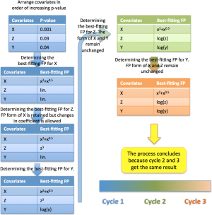
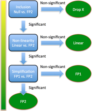
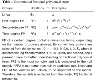
The first cycle is to build a multivariable model with all potential explanatory covariates (Figure 1). Alternatively, variables with P<0.25 or 0.2 in univariable analysis can be incorporated into the initial model. This is also the starting model for purposeful selection of covariates. All dichotomous and design variables are not subject to fractional polynomial (FP) transformation and are modeled with one degree of freedom. They are tested for their contribution to the model by using α1 (e.g., by Wald test). Continuous variables are modeled using closed test to examine whether they should be kept or removed using α1, and whether transformation should be performed using α2 (Figure 2). The closed test begins by comparing the best-fitting second-degree fractional polynomial (FP2) with null model (Table 1). The term is dropped if the test is non-significant. Otherwise the best-fitting FP2 is compared with the linear term. Linear term is adopted if the test is non-significant. Otherwise we continue to compare the best-fitting FP2 to the best-fitting FP1. If the test is significant the best fitting FP2 is adopted. Otherwise the best-fitting FP1 is adopted (6). The second cycle begins with a fit of model containing significant covariates, either in original or polynomial transformed form. All covariates are then examined in descending order of significance for their inclusion, exclusion and possible transformation. The procedure stops when two consecutive steps contain the same covariates with the same FP transformations.

Figure 1 A simple example illustrating the procedure of multivariable fractional polynomial method. Firstly, predictors are arranged in descending order of significance. The most important predictor is assessed by closed test for its inclusion and fractional polynomial (FP) function. The procedure proceeds sequentially for all predictors. The second cycle begins by examining the second predictor for its inclusion and FP function. Other predictors are kept in their FP form obtained from cycle 1. The procedure concludes when two cycles converge.

Figure 2 Closed test algorithm for choosing a fractional polynomial model with maximum permitted degree of 2 for a single continuous predictor. The first step is to determine whether a predictor should be included in a model. That is to compare models with and without FP2. If FP2 model is not better than null model, the predictor is dropped. Otherwise, we continue to compare FP2 with linear model. If FP2 is not better than linear one, we choose linear model. Otherwise, we continue to compare FP2 with FP1. If FP2 is not better than FP1, the FP1 model is chosen. Otherwise the FP2 model is chosen. FP, fractional polynomial.

Table 1 Illustration of fractional polynomial terms
Full table

Working example

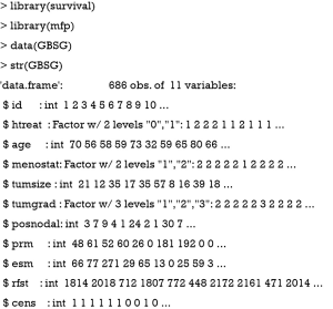
In this article, I use the German Breast Cancer Study Group (GBSG) database for illustration of MFP method. GBSG dataset in the mfp package contains 686 rows and 11 columns.

The variable id is to identify unique patient. Hormonal therapy (htreat) is a factor with two levels of no [0] and yes [1]. Menopausal status (menostat) is also a factor at two levels premenopausal [1] and postmenopausal [2]. Tumor size (tumsize) is a continuous variable measured in millimeter. Tumor grade (tumgrad) is an ordered factor at levels 1<2<3. Number of positive nodes (posnodal) is a continuous variable with integer values. Progesterone receptor (prm) is an integer variable measured in fmol. Estrogen receptor (esm) is an integer variable measured in fmol. Recurrence free survival time (rfst) is measured in days. Censoring indicator (cens) is an integer with 0 indicates censored and 1 for event.

Illustration of multivariable fractional polynomial (MFP) method

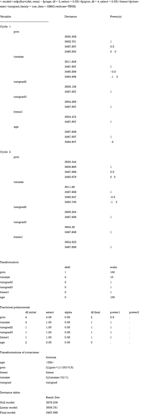
The GBSG dataset is a survival data and I construct the model with survival function. The Surv() function creates a survival object with the time and event as arguments. To make the model simple, only age and prm are selected for FP transformation. FP2 terms are allowed for prm and only FP1 is allowed for age. By default argument, FP2 is allowed for tumsize. The remaining variables htreat and tumgrad are linear because they are categorical. The model is built with Cox proportional hazard model by assigning “family = cox”. “verbose=TRUE” is to show variable selection details in output.

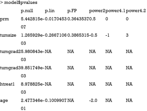
The first cycle begins by including all covariates into the model and their FP functions are examined. The best-ftting FP functions are shown in the output. For example, the power of best-fitting FP1 is 0.5 for prm, and the powers of best-fitting FP2 are -1 and 3 for tumsize. The statistical test is performed internally and not shown in the output. In cycle 2, age is dropped because the FP1 function is not significantly different from the null model (deviance: 3,494.907 vs. 3,497.698). Cycle 2 is the last cycle where the model converges. Transformation of each variable is shown. The variable prm is shifted by 1 and divided by 100 before FP transformation. FP functions of each variable remained in the model are shown in the output. Age is dropped. All variables are entered in linear form except that prm is transformed by FP1 with the power of 0.5. One can see P values of closed test procedure by the following code.

In the output, p.null corresponds to the test of inclusion (e.g., comparing best-fitting FP2 against null model); p.lin is the P value for the test of nonlinearity (comparing best-fitting FP2 against linear model) and p.FP is the test of simplification by comparing first degree (FP1) and second degree (FP2) transformations. The best-fitting FP1 power (power2) and best-fitting FP2 powers (power4.1 and power4.2) are also shown. The numbers 2 and 4 describe the corresponding degrees of freedom.

Next, users are interested in estimated coefficients for each transformed variable.

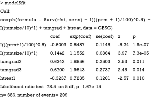
In the output of “model$fit”, one can see the final model is called by coxph() function. The coefficient for each transformed variable is shown in the table. Exponentiation of coefficient is the hazard ratio. The transformed variable is sometimes obscure to subject-matter audience. Visualization of how hazard ratio changes with variable of FP function is interesting.

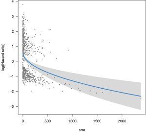
For the purpose of visualization of fitted regression model, I employ the visreg package. The visreg() function cannot directly receive returned object from mfp() and I refit the Cox model in the form exactly the same to that obtained from mfp(). Then the new model can be visualized using visreg() function (Figure 3). Sometimes, users are interested in visualization of survival curves at fixed covariates. For example, we can plot survival curves for patients with and without hormone therapy, given that the tumor size is 20 mm, progesterone receptor is 30 fmol, and tumor grade is 2 (Figure 4).

Figure 3 Visualization of non-linear model. Note that the variable prm is not linearly associated with log(hzazrd ratio).

Figure 4 Survival curves for patients with and without hormone therapy, given that the tumor size is 20 mm, progesterone receptor is 30 fmol, and tumor grade is 2.

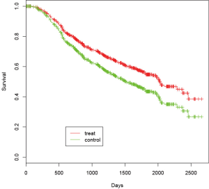
The survfit() function creates survival curves from previously fitted Cox model, here it is model$fit. The argument newdata specifies values of covariates to be plotted. The function legend() is used to add legend to make the plot more readable.

Summary

The article introduces how to perform MFP method by using mfp() function. Users can define which variable is subject to FP transformation and in what degree. The procedure firstly arranges potential predictors in order of decreasing significance (increasing P value). The purpose is to consider the relatively important variables before unimportant ones. Secondly, predictors are considered consecutively for their best-fitting FP function. The closed test algorithm is employed to choose a best-fitting FP function. Predictors of interest can be visualized by using visreg() function. Visualization of continuous predictors is important because coefficients of high-order terms are difficult to understand for subject-matter audience.

Acknowledgements

None.

Footnote

Conflicts of Interest: The author has no conflicts of interest to declare.

References

1. Zhang Z, Chen K, Ni H, et al. Predictive value of lactate in unselected critically ill patients: an analysis using fractional polynomials. J Thorac Dis 2014;6:995-1003. [PubMed]
2. Royston P, Ambler G, Sauerbrei W. The use of fractional polynomials to model continuous risk variables in epidemiology. Int J Epidemiol 1999;28:964-74. [Crossref] [PubMed]
3. Royston P, Altman DG. Regression Using Fractional Polynomials of Continuous Covariates: Parsimonious Parametric Modelling. Applied Statistics 1994;43:429-67. [Crossref]
4. Royston P, Sauerbrei W. Building multivariable regression models with continuous covariates in clinical epidemiology--with an emphasis on fractional polynomials. Methods Inf Med 2005;44:561-71. [PubMed]
5. Sauerbrei W, Royston P, Binder H. Selection of important variables and determination of functional form for continuous predictors in multivariable model building. Stat Med 2007;26:5512-28. [Crossref] [PubMed]
6. Marcus R, Eric P, Gabriel KR. On closed testing procedures with special reference to ordered analysis of variance. Biometrika 1976;63:655-60. [Crossref]