A gentle introduction to artificial neural networks

Introduction

Artificial neural networks (ANN) mimic human brain in processing input signals and transform them into output signals (1). It provides powerful modeling algorithm that allows for non-linearity between feature variables and output signals. ANN is a kind of non-parametric modeling technique, which is suitable for complex phenomenon that investigators do not know underlying functions. In other words, ANN is able to learn from data without specific function assumptions. The article firstly provides some basic knowledge on ANN, and then shows how to conduct ANN modeling with simulated data. Predicting performance of the ANN is compared to that of generalized linear model.

Understanding ANN

ANN works in a very similar way to human brain. In structure, human brain is made up of neurons and there are approximately 85 billion neurons in human brain (2). The dendrites of a neuron receive input signals from environmental stimulation or up-stream neurons. Signal is processed in the cell body and transmits along axon to the output terminal. The output signal may be received by down-stream neurons or by the function organs such as muscles to make reaction. A single artificial neuron works in a similar way. Feature variables, also known as predictors, input variables and covariates, are input signals that provide information for pattern recognition. Each feature variable is weighted according to its importance (3). This work is done by dendrites in the biological nervous system. The weighted signals are summed and processed by activation function. The signal processing procedure can be mathematically expressed as:

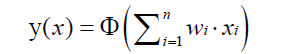
where y is the output signal, Φ() is the activation function, x is input variables and w is weight assigned to each input variables. Suppose there are n input variables. To better understand ANN, it can be compared to the regression model. Each input variable is in analogue to the predictors of a regression model. Weight is actually the coefficient of each predictor.

In ANN topology, input nodes receive feature variables from raw data and the output node applies activation function to combined information from input nodes. The nodes are arranged in layers (3). For example, all input nodes constitute one layer. If a network only contains input and output nodes, it is termed single-layer network, or skip-layer units. Such network is commonly used for simple classification in which the outcome pattern is linearly separable. More complex task should be done with multilayer network that adds one or more hidden layers to the single-layer network. In our example, we allow for one hidden layer to be added to the network.

Working example

To illustrate how to build ANN with R, I created a simple example. The dataset is made of two input variables x1 and x2, and one output variable y with three levels. The dataset is generated by the following syntax.

To simulate a multinomial outcome variable, we created two logit functions, namely logit1 and logit2 (4). The three-level output contains one reference level, and the remaining two is compared to the reference level. Then the probability of each level can be computed from input features. Here quadratic terms of input variable are applied. For each observation, the level with the largest probability is assigned value one and the remaining two levels are coded by zero. The last line combines these variables into a data frame.

To take a look at the dataset, I employ the qplot() function. If you have not installed ggplot2 package, install it before running the library() function (5).

Figure 1 plots x1 against x2, which constitutes a two-dimension feature space. It appears that the three classifications are not linearly separable, which is as expected because I constructed output classifications with quadratic terms. In particular, class 3 is embedded between class 1 and 2.

Figure 1 Distribution of observations in the two-dimension feature space. Classifications are denoted with dot colors. The three classifications are not linearly separable, which is as expected because output classifications are constructed with quadratic terms.

ANN training and visualization

ANN training can be easily done using the nnet() function. The original cohort is split into training and test sets. Because the observations in data are randomly arranged, the first 700 cases are used as training set and the remaining 300 are used as test set.

Up to now, the data are well prepared for ANN training. In most situations, the feature variables should be scaled before being passed to the nnet() function. However, this step is not necessary because our feature variables are created in the same scale.

The above code created an object of class “nnet” and stored with the name of annmod. The first argument of nnet() function is a data frame of feature variables and the second argument is a vector of response variable. The size argument defines the number of units in the hidden layer.

The visualization function of ANN is not included in the nnet package. Fortunately, there is a function plot.nnet() that is very powerful in plotting the neural network. It also allows for customization of the graph with varieties of options. To install the package into your workspace, you need to install the devtools package. It contains package development tools for R.

The plot.nnet() function runs in the following way.

The first argument of the function is an object of “nnet”. Transparency of connections is determined by the alpha.val argument whose value ranges between 0 and 1. The color of positive connections is determined by pos.col argument and here I make it green. Similarly, the negative connections are depicted with red color. Figure 2 is the ANN plot showing nodes and connections of the network. There are two input nodes named I1 and I2, transmitting information from feature variables x1 and x2. Weights are assigned to each of the connections between input nodes and hidden nodes. The green and red colors represent the positive and negative weights, respectively. B1 is the bias applied to hidden neurons. Finally, signals are transmitted to the output neurons which are denoted by O1 through O3. Similarly, there are weights and bias applied to the output neurons.

Figure 2 Artificial neural networks plot showing nodes and connections of the network. There are two input nodes named I1 and I2, transmitting information from feature variables x1 and x2. The green and red colors represent the positive and negative weights, respectively. B1 is the bias applied to hidden neurons.

Prediction with ANN

Training of the ANN is only the first step of our task. More important work is prediction on future observations with the trained model. Like prediction with other models, the predict() function works well with ANN. The first argument is an object of “nnet”. The second argument is a data frame containing feature variables. Because the response variable in our example is a factor variable with three levels, the type of output is “class”.

To examine the predictive accuracy of the ANN model, I created a confusion matrix as shown in the output of table() function (6). The diagonal of the matrix shows correctly classified numbers. Alternatively, the classification of ANN model can be evaluated using average accuracy (7). I write a function called accuracyCal() to perform the calculation in the following syntax.

With this function we can easily calculate a series of average accuracy by varying the number of units in the hidden layer. In the following syntax, a number of 30 is passed to the function, which in turn returns a series of average accuracies for ANN with the number of hidden layer units ranging from 1 to 30. Visualization of how average accuracy varies with the size parameter can be performed with generic plot() function.

Figure 3 plots average accuracy against number of units in hidden layer. It appears that the accuracy reaches its largest value when the number of units is between 5 to 10.

Figure 3 Plotting average accuracy against number of units in hidden layer. It appears that the accuracy reaches its largest value when the number of units is between 5 to 10.

Comparison with generalized linear model

The same task can be done with generalized linear model. For classification of outcome variable with three levels, the multinomial logistic regression model is a choice. The function multinom() shipped with nnet package can do the work.

The confusion matrix shows that the predictive performance of generalized linear model is not significantly poorer than ANN. Next we continue to calculate the average accuracy.

The average accuracy is 0.82, which is slightly lower than that obtained by ANN with size equal to 6.

Summary

The article introduces some basic ideas behind ANN. It is in analogue to the human brain. There are input and output signals in ANN. Input signals are weighted before reaching output nodes according to their respective importance. Then the combined signal is processed by activation function. I simulated a simple example to illustrate how to build a simple ANN model using nnet() function. This function allows for one hidden layer with varying number of units in that layer. The basic structure of ANN can be visualized with plug-in plot.nnet() function. The plot function is powerful that it allows for varieties of adjustment to the appearance of the neural networks. Prediction with ANN can be performed with predict() function, similar to prediction with conventional models. Finally, the prediction power of ANN is examined using confusion matrix and average accuracy. It appears that ANN is slightly better than conventional linear model.

Acknowledgements

None.

Footnote

Conflicts of Interest: The author has no conflicts of interest to declare.

References

1. Wesolowski M, Suchacz B. Artificial neural networks: theoretical background and pharmaceutical applications: a review. J AOAC Int 2012;95:652-68. [Crossref] [PubMed]
2. Lantz B, editor. Machine learning with R. 2nd ed. Birmingham: Packt Publishing, 2015:1.
3. Haykin SO, editor. Neural networks and learning machines. 3rd ed. New Jersey: Prentice Hall, 2008.
4. Hosmer DW Jr, Lemeshow S, Sturdivant RX, editors. Applied logistic regression. 3rd ed. Hoboken, NJ: Wiley, 2013:1.
5. Wickham H, editor. ggplot2: elegant graphics for data analysis. New York: Springer-Verlag, 2009.
6. Stehman SV. Selecting and interpreting measures of thematic classification accuracy. Remote Sensing of Environment 1997;62:77-89. [Crossref]
7. Hernandez-Torruco J, Canul-Reich J, Frausto-Solis J, et al. Towards a predictive model for Guillain-Barré syndrome. Conf Proc IEEE Eng Med Biol Soc 2015;2015:7234-7.