Variable selection in Logistic regression model with genetic algorithm

Introduction

Variable or feature selection is of vital importance in building a multivariable regression model. The primary purpose of variable selection is to incorporate clinically relevant and statistically significant variables into the model, while excluding noise/redundant variables (1,2). There are many procedures for this purpose such as purposeful selection, best subset and stepwise regression, association rules techniques, particle swarm optimization, etc. These procedures have been proven to be powerful in model building, and are widely used. However, none of these procedures are panacea, especially in the era of big data when a huge number of variables are available. The purposeful selection of variables usually involves univariate testing to screen variables that are significantly associated with the outcome of interest. Then a regression model is built on these variables. However, such a procedure may overlook some important variables which work together to take effect, but they do not reach statistical significance level when tested independently. The best subset procedure can solve this problem because it tests all the possible combinations of the candidate variables (3). However, this procedure can be useful in a dataset with small number of variables, but may not be the best choice for a large number of variables. For example, when there are 50 candidate variables, the total number of models is 2⁵⁰–1, which is obviously unmanageable with modern computers (2). Stepwise approach is another widely used method, but it is a local search process that it ultimately converges to local optima (4).

Genetic algorithm (GA) is a heuristic search algorithm mimicking the process of biological evolution and natural selection (5,6). In Darwin’s theory, the population can evolve by selection, crossover and mutation. In the process, the fittest individuals will survive and reproduce whereas the weaker ones will be eliminated from the population. GAs create random populations of artificial individuals (chromosomes in GAs terminology) that are evaluated by a mathematical fitness function. When the fittest chromosomes are selected, reproduced, crossed, and mutated along many generations, the artificially evolved chromosomes are quite well adapted to the mathematical fitness function. GAs have been successfully applied to solve optimization problems, both for continuous (whether differentiable or not) and discrete functions. Variable selection for logistic regression model can be regarded as an optimization problem, and thus can be solved by GAs (7-10). This article aims to provide a tutorial on how to implement GAs for variable selection. Since the logistic regression model is the most widely used method in clinical researches, because in most cases, the dependent variable is categorical (e.g., diagnosis), it will be considered as a working example. The code can be easily extended to other types of generalized linear models, owing to the availability of a large amount of R packages for these functionalities.

Basic ideas underlying GA

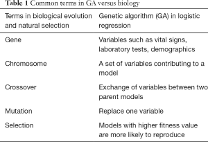
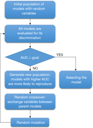
The principles of evolution and natural selection are the stepping stones of GA (5,11). In biology, gene is a unit of heredity that can be transferred from parents to offspring and is held to determine some characteristic of the offspring (12). A chromosome is comprised of genes. In an analogy, a clinical variable can be considered as a gene (Table 1), and a set of clinical variables constructing a regression model can be considered as a chromosome. The chromosome size specifies the number of variables for a model. For example, if the chromosome size is 5, there will be five different variables in each model. The GA begins with a population of a random set of models. A fitness function is applied to evaluate each model in the population. For logistic regression models, the fitness function can be the discrimination as represented by the area under the receiver operating characteristic curve (AUC). It is noteworthy that AUC combines in a unique value both the sensitivity and specificity of a model. The traditional evaluation system for AUC (i.e., 0.9–1.0—excellent; 0.8–0.9—good; 0.7–0.8—fair; 0.6–0.7—poor; 0.5–0.6—failure) is usually used to assess the performance of each classifier. To finish the evolving process, the AUC is compared to a goal (A main open question that cannot be simply answered without a complex combinatorial optimization approach concerns the choice of the values to be set for the algorithms parameters of GA. For the sake of simplicity, in this paper we heuristically chose them, although in future work this issue needs to be considered). If the goal is reached, the model is selected and the evolution process stops. If the goal is not reached in the current generation, the population of models will continue to evolve. Here, the current population act as the parent population and the next generation is the offspring. Similar to the biological evolution, models with greater fitness in parent population have more chance to reproduce. The replicated chromosome will undergo crossover and mutation to produce diversity, allowing the offspring to have more chance to reach the fitness goal. The cycle continues until either the fitness goal or the maximum number of generations is reached (Figure 1).

Table 1 Common terms in GA versus biology
Full table

Figure 1 Flow chart of genetic algorithms. At the outset, a population of models is created randomly, and they are evaluated for their fitness. In this example, the discrimination of the area under the receiver operating characteristics curve (AUC) is used as the fitness value. If there is a model reaching the fitness goal, the model is selected and the evolutionary process discontinues. Otherwise, the parent generation proceeds to reproduce offspring, with models of higher AUC more likely to reproduce. There are crossover and mutation mechanisms to expand the reservoir of models.

Working example

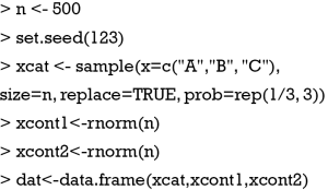
Here we simulate a dataset to illustrate of how to perform variable selection with GA. The R code for generating the dataset is shown below (R version 3.3.2):

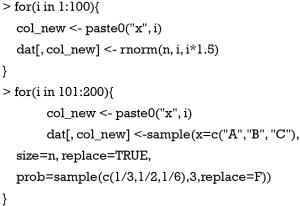
The first line specifies the number of observations as 500. The set.seed() function allows the results to be reproducible across computers. The xcat variable is a categorical variable with three levels A, B and C, and the three levels have the same probability of occurrence. Two continuous variables xcont1 and xcont2 are created assuming normal distribution. However, if the number of observations is fairly large (≥100), as in this case, then deviations from normality do not matter too much because of the central limit theorem (CLT). Then, the three variables are coerced into a data frame. Assuming that the three variables are associated with the outcome variable, we also created 100 noise variables (50 categorical and 50 numeric) that are not associated with the outcome variable, and add them to the data frame.

A total number of 100 noise variables are generated using for loop, comprising 50 categorical and 50 numeric variables. The next code is to produce the outcome variable y which is a binary categorical variable.

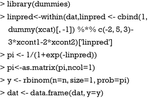
The linpred object is a linear combination of predictors. Note that only three variables xcat, xcont1 and xcont2 contribute to the linear predictor. Then the linear predictor is converted to the probability by using the inverse logit function. The outcome y is produced by assuming a binomial distribution, although, in specific cases, other discrete distributions may be taken into account. The last line combines dat and y into the final data frame. Such a data frame is usually the start of data analysis in real clinical research practice.

The galgo package

Several R packages exist such as GA (13), genalg and GenAlgo that can be used for implementing GA. However, in this tutorial we will use the galgo package (v1.2-01), a popular tool in bioinformatics (14). The galgo package contains plenty of useful tools for the visualization of GA process. Furthermore, the objects can be extended and all functions can be overwritten, allowing users to adapt functions in the galgo package to their own needs. There is a good tutorial available on the web for the comprehensive description of the package (http://bioinformatica.mty.itesm.mx/Galgo). Also one may consult R documents which can be invoked by calling the help() function. As we already mentioned, since logistic regression is the most widely used statistical method in clinical researches, the present tutorial focuses on the use of the galgo package to build a logistic regression model.

Define the fitness function

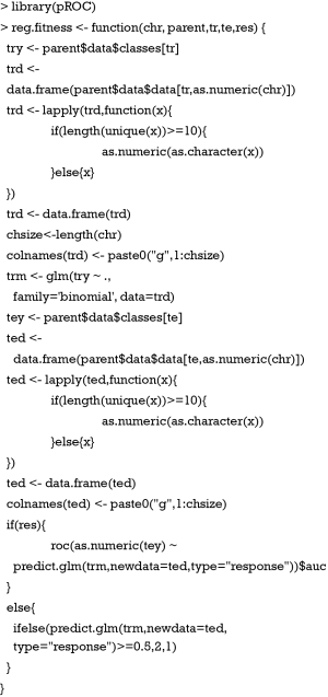
The core to variable selection is the fitness function because it judges how good one model fits to the data. There is a variety of methods to judge the fitness of a model such as the Homser-Lemeshow goodness of fit test (for logistic regression models), the discrimination, the Akaike information criterion (AIC) and Bayesian information criterion (BIC) (4). In this article, the discrimination method is used to evaluate the goodness of a logistic regression model. Discrimination is quantitatively assessed by the AUC (15,16). The pROC package is employed to compute the statistic (17). The fitness function is constructed by the following code.

The fitness function requires the prototype of the form function (chr, parent,tr,te,res), where chr represents the chromosome to be evaluated. parent is the BigBang object that will be created by the wrapper function configBB.VarSel() in the next section. tr is the vector of samples (rows) that is used as training, and te the samples that must be used as test. The res argument controls the format of the returned object. For res=0, a vector of the same length as the testing sample containing predicted class will be returned; otherwise, the returned value is an AUC of the model calculated in the testing dataset.

The outcome variable in the training dataset can be extracted by “parent$data$classes[tr]”. The predictors of the training dataset are stored in the object trd. Since in the BigBang object, the original data frame is transposed so that all variables are converted to character vectors, it is necessary to convert the numerical variables back to class of numeric (variable type). The variables are renamed to g1, g2, g3, g4 and g5 in the fitness function. In this tutorial, as an example, we restrict five variables being selected to construct a logistic regression model, and the task of the fitness function is to evaluate the fitness of the model. In this respect, the fitness function has nothing to do with the variable selection procedure. Next, the logistic regression model is built with the glm() function in a conventional way. The test dataset is extracted in the same way as that for the training dataset. Finally, the if-else function is employed to return different results. As mentioned above, if the res argument is 0, the returned object is a vector containing class membership for each individual in the test dataset. Otherwise, the fitness function will return an AUC value reflecting the discrimination of the model.

The BigBang object

The evolution will stop by either the preset maximum number of generation or the fitness goal is reached. As a result, there could be a solution to the problem (the fitness goal is reached) or no solution at all. In our example, one evolution may result in a model with the preset discrimination or not. More importantly, the solution may be a local maximum. Thus, it is necessary to implement a large amount of evolutions. The BigBang object is an attempt to use more information of a large collection of solutions instead of a unique solution. The BigBang object can be created using the wrapper function configBB.VarSel() as follows:

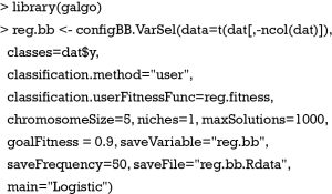
The data argument is a data frame with samples (patients) in columns and variables in rows, which is a transposed format of the conventional data frame. Note that the outcome variable is not provided in the data argument, but it is provided separately in the classes argument. There are many classification methods shipped with the galgo package such as support vector machines (SVMs), neural networks (NNs) and nearest neighbors. Here the user-defined function which we were previously created is used. The user-defined function is given in the classification.userFitnessFunc argument. The chromosome size is set to 5, indicating that the models will consist of 5 variables. The maximum number of solutions is 1,000, which is considered as the default value. The fitness goal is set to be 0.9 as an example, indicating that if a model with AUC equal or greater than 0.9 is evolved the evolution process will stop, and the program will go to another cycle of search for solutions. After the BigBang object is properly configured, the “blast” procedure has to be started to collect chromosomes (models) associated with high AUC.

The real time evolutionary process can be monitored after running the blast() function. An example of the output is shown above lines starting with [e] represent the evolutionary process. The first line shows the fitness goal, the minimum and maximum number of generations. In the example, the minimum number of generation is 10, and the maximum number is 200. The second column shows the elapsed time. In the example, the first 20 generations take 20 s to evolve. The third column shows the current number of generation (refreshed every 20 generations by default). The “Fitness” column shows the current best fitness, along with the percentage relative to the fitness goal in the “%Fit” column. The “[NextGenerations]” column shows the behavior of the next generation. A “.” symbol indicates that the maximum fitness of the current population has not changed, “+” means it has increased and “-” means it has decreased. The “G” symbol may sometimes appear, indicating that the fitness goal has been reached but the minimum number of generation has not been reached. The numbers following “FINISH” is the indices of variables constituting the best-fit chromosome.

The last line starting with [Bb] shows the current collection of solutions in the whole BigBang object. In the example, the number of evolutions is 49 and the number of evolutions that have reached goal fitness is 49. The “Sol Ok” indicates that the current evolution reaches goal fitness. The best fitness is 0.94737, along with its percentage 105.26% relative to the fitness goal. The number of generations required to reach the goal fitness is 83, and it takes 84.986 s. The accumulated process time spent in all evolutions is 3,109 s. The time 3,127 s is the accumulated real time, including the time spent on saving objects and other system delays. The remaining time required to complete the total [1,000] evolutions is 59,410 s (16 h 30 min 10 s). The evolutionary process can be visualized with plots.

The result is shown in Figure 2. A total of 50 chromosomes (models in logistic regression term) are collected, including those with and without solutions. The frequency of variables that are present in the models is shown in the top plot. The top 7 variables are in black color and named. The top 50 variables are shown in other colors. In the example, the three variables remarkably dominate the other variables in the frequency of appearance, because we have deliberately modeled the first three variables to be related to the outcome variable y. The middle plot shows the stability of the rank of the 50 top variables. In other words, it is to show whether the frequency of a variable remain stable with accumulating chromosomes. When rank colors change frequently for a variable, the rank of the variable is unstable. From the plot, it can be seen that the first three variables show stable rank (always in black color), but the remaining variables change their rank colors frequently. The vertical axis comprises of two parts: variable frequency and the number of evolutions. The horizontal axis represents the variable indices. The bottom plot shows the distribution of the number of generations required for an evolutionary episode to reach the fitness goal. It appears that in average a number of 50 generations is required for a GA process to reach the fitness goal.

Figure 2 The evolutionary process is tracked with plots. The top plot shows the frequency of variables occurred in the selected models. The top 7 variables are in black and the remaining top 50 variables are colored. The middle plot shows the rank stability of a variable. If a variable shows many changes in color, it is not stable and more evolutions are required. In this example, the first three variables xcat, xcont1 and xcont2 are considered to be stable. The plot at the bottom shows the distribution of the number of generations required for each GA evolution. Note that there are 200 generations at maximum because we set the maximum generation to be 200.

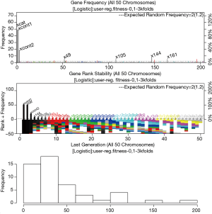
The fitness of all chromosomes can be visualized with fitness plot, which can be plotted using the following code.

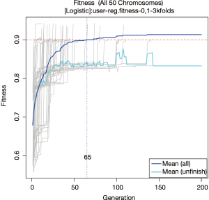
The plot is shown in Figure 3. The fitness values (AUC in the example) of all GA evolutionary processes are traced across generations (grey thin lines). The blue curve shows the average fitness value across generations for all chromosomes, and the light blue curve is for chromosomes that have not reached the fitness goal in current generation. If all chromosomes reach a goal before 200 generations, the two curves will converge at the end. However, it is not the case in the present example. The plot shows that a solution can be reached in 65 generations in average. This can be used to limit the searches in future runs to save time.

Figure 3 The fitness value changes over evolution. Each thin grey line represents an episode of evolution and there are 50 evolutions in this example. The blue thick line shows the mean fitness value for all evolutions and the light blue line represents the mean value for the unfinished evolutions at current generation number. In average, 65 generations are needed to reach the fitness goal.

Variable composition of collected model can be visualized in terms of top-ranked variables (Figure 4).

Figure 4 Gene overlap plot shows how genes appear together in a chromosome (model). Chromosomes are ordered by the presence of top-rank genes. Note that the top 3 genes are present in all chromosomes.

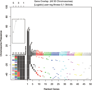
The vertical axis shows all models (chromosomes) being collected and the horizontal axis represents the variables ranked by their frequency. The models are first ordered by the presence of the most frequently occurred variables (e.g., here it is xcont1), then by the presence of the second mostly frequently occurred variables (xcat), and so on. Thus, models with similar top-ranked variables are stacked together. Of the 203 variables being screened, the top 50 are displayed in the plot. The xcont1 is present in all 50 models, xcat is present in 49 models, and xcont2 in 20. Recall that the outcome variable y is composed of these three variables and therefore it is expected to find these variables in the top ranked ones. In general, from the plot, it can be seen which variable is usually combined with the top variables.

The dependency of each variable can be visualized using network plot (Figure 5).

Figure 5 Gene interaction in models. The numbers in the figure represent the order number of variables. For example, the 1, 2 and 3 represent the variables xcont1, xcat and xcont2. The thickness of lines represents the strength of dependency between two variables.

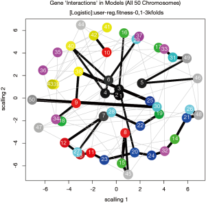
The number is the order number of variables. For example, the 1, 2 and 3 represents the xcont1, xcat and xcont2 variables. The thickness of lines represents the strength of dependency between two variables. By default, only two dependency relationships are displayed.

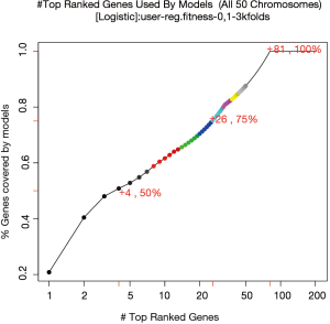
Figure 6 shows the percentage of top-ranked genes used by models. The top 4 genes account for 50% of all genes used in the 50 models, and the top 26 genes account for 75%. The 50 models have used 81 out of the 203 genes (variables) in the pool.

Figure 6 Top-ranked genes used by the model. The top 4 genes account for 50% of all genes used in the 50 models, and the top 26 genes account for 75%. The 50 models have used 81 of the 203 genes in the pool.

The overall accuracy of the selected models

After obtaining the 106 models from the GA process, the overall accuracy of these models need to be assessed. By default, the original dataset is split into training and test datasets at 2:1 ratio. The training set is used for model development and the test set is used to assess the model accuracy. A confusion plot can be produced by the following code.

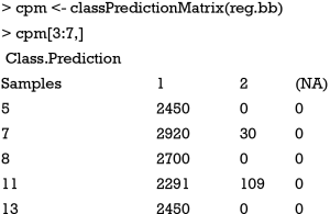
The output of the function is shown in Figure 7. Here only 50 chromosomes are used for saving the computation time. Users may not reproduce the plot exactly due to random process. The horizontal line represents the samples sorted by original class. Note that there are 219 samples in class 1 and 281 in class 2. All samples have been predicted. The bars represent the percentage of models that classify each sample in a given class. Samples in the first column (black) belong to class 1, and they are correctly identified by models for 81.7% of the times and wrongly classified as “class 2” for 18.3% of the times. The plot also displays the sensitivity and the specificity of the prediction. The numeric format of the confusion matrix can be obtained using the following code.

Figure 7 Class confusion plot shows the predicted and observed class membership for each individual. The bars represent the percentage of models that classify each sample in a given class. Samples in the first column (black) belong to class 1, and they are correctly identified by models for 81.7% of the times and wrongly classified as “class 2” for 18.3% of the times.

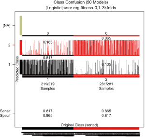
For sample 7, the chromosomes predicted it as class 1 for 2,920 times and as class 2 for 30 times. It makes 2,950 predictions for the sample. The number of predictions can be calculated as the number of splits into training and test datasets divided by 3, and then multiplied the number of chromosomes. In the present example, the total number of predictions made in the test set is 50*150/3=2,500 in average.

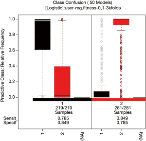
Similar information can be represented in a confusion box plot.

Figure 8 plots the relative frequency of predicted class on the vertical axis versus the observed class on the horizontal axis. It shows that most models can correctly predict the class membership.

Figure 8 Box plot of class confusion. The vertical axis shows the relative frequency of predicted class, and the horizontal axis shows the observed class membership.

Splits of the sample

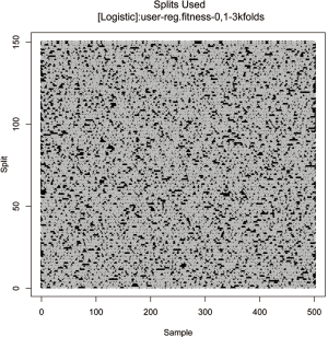
The original sample (n=500) is split into the training and test sets in 2:1 ratio (first-level split). By default, the data is randomly split for 150 times with the same ratio of training to test sets. The training set is then undergone k-fold cross validation during the GA process (second level split). The evolutionary process only employs the second-level split. The first level split is used for error estimation outside the evolutionary (blast) process. However, this can be controlled in galgo object (see R document). The split can be visualized with the following code.

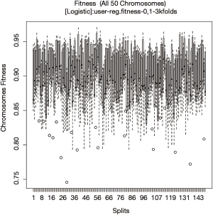
The vertical axis shows the 150 random splits and the horizontal axis shows the 500 samples (Figure 9). The plot may not be useful because the splits are randomly performed and it is only needed to know the number of splits, and the ratio of training to test samples. However, the split plot may help to understand how the galgo works to split data. The following code produce a plot showing fitness values across different split patterns.

Figure 9 The plot shows how the whole population is split into training and test datasets. The vertical axis shows the 150 random splits and the horizontal axis shows the 500 samples.

There are 150 random splits in total and the fitness of each chromosome is evaluated in the test set of each of the 150 splits (Figure 10). The fitness values of all chromosomes evaluated with a given split pattern are aggregated in a box. The plot can help to check whether the fitness values of chromosomes are split-dependent.

Figure 10 Fitness values of chromosomes evaluated in each split pattern. There are 150 random splits in this example and the fitness of each chromosome is evaluated in the test set of each of the 150 splits. The fitness values of all chromosomes evaluated with a given split pattern are aggregated in a box.

Select variables which are important to the model

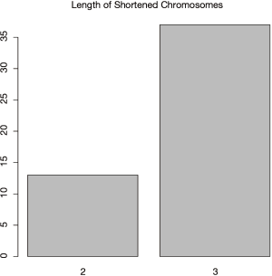
In real clinical research practice, the number of variables that are of great importance to the model is usually unknown. Investigators may set out to define a fixed number of variables for a given model and then select the important ones from the model pool. In the present example, 5 variables are defined for each model in the GA process. Since the BigBang object has run a total of 50 cycles of evolutionary process, there are 50 best-fit models being selected. Although there are only 5 variables in a given model, the number of variables can be much larger in the 50 models. Variable selection can be performed by the backward selection, in which a variable is removed from the model and the classification accuracy of the shorter resulting model is assessed. If the accuracy of the shorter model is not significantly reduced, another cycle is performed. Otherwise, the variable is left in the model and the program proceeds to another cycle of elimination. The backward elimination procedure influences the model sizes which can be evidenced by the following code.

The result shown in Figure 11 indicates that most of the models (>35) require 3 variables to keep a high accuracy, and only 13 models retain 2 variables.

Figure 11 Length of shortened chromosome. It is noteworthy that most of the models (>35) require 3 variables to maintain a high predictive accuracy, and only 13 models require 2 variables.

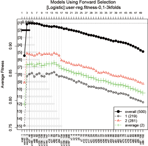
The GA procedure provides a large collection of models and sometimes investigators are interested in a representative model that has the highest prediction accuracy. The frequency of variables in the collection of models can be employed as criteria for inclusion in a forward selection procedure.

The function automatically produces a plot showing the variable selection process (Figure 12). The vertical line is the fitness value (AUC in the present example), and the horizontal line represents the variables sorted in descending order of gene frequency. For the overall prediction accuracy, the second model comprising 4 variables xcat, xcont1, xcont2 and x37 appears to have the highest accuracy (AUC =0.9419). 14 more models whose fitness values are 99% as close to the best model are displayed in the plot.

Figure 12 Models using forward selection. The vertical line represents the fitness value (AUC in this example), and the horizontal line represents the variables sorted in descending order of gene frequency. For the overall prediction accuracy, the second model comprising 4 variables xcat, xcont1, xcont2 and x37 appears to have the highest accuracy (AUC =0.9419). Fourteen more models whose fitness values are 99% as close to the best model are displayed in the plot.

Conclusions

GA approach is appropriate for finding solutions that require efficient searching of a subset of features to find combinations that are near optimal for solving high-dimensional classification problems, especially when the search space is large, complex or poorly understood. Clinical diagnosis and prognosis can be treated as a classification problem, and selection of an optimized set of features can be the key of the accuracy. Logistic regression as a classifier has gained its popularity in clinical research. This tutorial demonstrated a way of applying GA for feature selection in combination with logistic regression for classification. It uses a simulated data set as an example and the result has shown the capacity of GA for selecting the best or near best classification model with a small set of variables. When applying to real clinical data, it can help discover the knowledge from a complex situation and help researchers understand the mechanism of diseases, so that benefit the medical research outcome. The tutorial gives a guide of how to use the galgo package in a way that was considered as the most relevant to medical researches. The parameters in the scripts can be chosen with preference, and many other functions are also included. Also other R packages that implement GA can be tried instead of galgo for further interest.

Acknowledgements

Funding: Z Zhang was supported by Zhejiang provincial natural science foundation of China (LGF18H150005) and V Trevino by CONACyT.

Footnote

Conflicts of Interest: The authors have no conflicts of interest to declare.

References

1. Tolles J, Meurer WJ. Logistic Regression: Relating Patient Characteristics to Outcomes. JAMA 2016;316:533-4. [Crossref] [PubMed]
2. Kiezun A, Lee IT, Shomron N. Evaluation of optimization techniques for variable selection in logistic regression applied to diagnosis of myocardial infarction. Bioinformation 2009;3:311-3. [Crossref] [PubMed]
3. Zhang Z. Variable selection with stepwise and best subset approaches. Ann Transl Med 2016;4:136-6. [Crossref] [PubMed]
4. Paterlini S, Minerva T. Regression model selection using genetic algorithms. In: Munteanu V, Raducanu R, Dutica G, et al. editors. Recent Advances in Neural Networks, Fuzzy Systems & Evolutionary Computing. Iasi, Romania: WSEAS Press; 2010:19-27.
5. Lucasius CB, Kateman G. Understanding and using genetic algorithms Part 1. Concepts, properties and context. Chemometrics and Intelligent Laboratory Systems 1993;19:1-33. [Crossref]
6. Escalona-Vargas D, Murphy P, Lowery CL, et al. Genetic algorithms for dipole location of fetal magnetocardiography. Conf Proc IEEE Eng Med Biol Soc 2016;2016:904-7. [PubMed]
7. Vandewater L, Brusic V, Wilson W, et al. An adaptive genetic algorithm for selection of blood-based biomarkers for prediction of Alzheimer's disease progression. BMC Bioinformatics 2015;16 Suppl 18:S1. [Crossref] [PubMed]
8. Vinterbo S, Ohno-Machado L. A genetic algorithm to select variables in logistic regression: example in the domain of myocardial infarction. Proc AMIA Symp 1999.984-8. [PubMed]
9. Gayou O, Das SK, Zhou SM, Marks LB, et al. A genetic algorithm for variable selection in logistic regression analysis of radiotherapy treatment outcomes. Med Phys 2008;35:5426-33. [Crossref] [PubMed]
10. Tolvi J. Genetic algorithms for outlier detection and variable selection in linear regression models. Soft Computing 2004;8:527-33. [Crossref]
11. Holland JH. Genetic Algorithms and Adaptation. In: Selfridge OG, Rissland EL, Arbib MA. editors. Adaptive Control of Ill-Defined Systems. Boston, MA: Springer US; 1984:317-33.
12. Holland J. Biology's gift to a complex world. Scientist 2008;22:36-43.
13. Scrucca L. GA. A package for genetic algorithms in R. Journal of Statistical Software 2013;53:1-37. [Crossref]
14. Trevino V, Falciani F. GALGO: an R package for multivariate variable selection using genetic algorithms. Bioinformatics 2006;22:1154-6. [Crossref] [PubMed]
15. Sun L, Wang J, Wei J. AVC: Selecting discriminative features on basis of AUC by maximizing variable complementarity. BMC Bioinformatics 2017;18:50. [Crossref] [PubMed]
16. Wang B. Variable selection in ROC regression. Comput Math Methods Med 2013;2013:436493. [PubMed]
17. Robin X, Turck N, Hainard A, et al. pROC: an open-source package for R and S+ to analyze and compare ROC curves. BMC Bioinformatics 2011;12:77. [Crossref] [PubMed]