Subgroup identification in clinical trials: an overview of available methods and their implementations with R

Introduction

Randomized controlled trials (RCT) are the cornerstone of the evidence based medicine, providing strong evidence for decision-making in medicine and healthcare. Methodologically, RCT is a robust study design employed to test the biological efficacy of a novel intervention as compared with the control one using clinical and laboratory outcome measures (1). Well-designed RCTs should be conducted in a homogeneous study population, which is a crucial aspect to evaluate the efficacy of an intervention in RCTs. Applying a strict inclusion/exclusion criteria is the commonest approach to enroll participants with similar characteristics.

Although such experimental design is appropriate to assess the treatment efficacy with good internal validity, its external validity has been criticized mainly because the characteristics of study patients from distinct RCTs may differ importantly jeopardizing the generalization of the results. Thus, the concept of real world study (RWS) aligning pragmatic trials with clinical practice comes into scientific community (2). No matter how strict is the inclusion/exclusion criteria of a RCT, the baseline characteristics of the study population can differ considerably. As a result, the effect size of a certain intervention can be significantly influenced by the heterogeneity of the study population. For instance, given a RCT with neutral effect, there can be a beneficial effect for a specific subgroup of patients but not for others participants. The findings of the original design of the RCT report only the average effect across heterogeneous subgroups. In some cases, clinical investigators may want to overcome the negative results of the RCT by reporting analysis of patient subgroups. Although such a post hoc analysis is at high risk of spurious findings, this can still be an option to generate some interesting findings that warrant further experimental trials to confirm the subgroup analysis.

A variety of methods have been developed for the identification of subgroups of participants in RCTs, including penalized regression model with interaction terms and tree based partitioning. These methods will be discussed in the following sections. In a recent tutorial paper, Lipkovich and colleagues have made a comprehensive review of these methods (3). Herein, we aim to review some of these methods and provide specific R code (R version 3.4.3), as well as detailed explanations, for the performance of these methods.

Working example

Here we generate an artificial dataset for the illustration of the methods for identifying subgroups of participants in RCTs. The study population is simulated with subgroups which have opposite treatment effects. The data structure can be outlined with the equation:

where z is a continuous outcome, which can be transformed to binary outcome y. A binary outcome variable is subject to logit transformation to establish a linear link with covariates. I() denotes the indicator function, which returns 1 if the logistic function is true and 0 otherwise. The R code for generating the dataset is as follows:

The above code generates a dataset with a sample size of 2000. Suppose there are four baseline variables being collected, which are denoted as x1, x2, x3 and x4. Only x1 and x2 are correlated with the outcome variable y. x3 and x4 are noise variables. The variable t represents the treatment variable, which is typically a binary factor variable comprising two categories (e.g., A=active treatment vs. C=control). Considering a hypothetical RCT fails to identify the expected beneficial health effect of the treatment intervention as compared to the control.

The above code performs univariable analysis to examine whether there is statistical difference between treatment and control arms in the binary outcome y. The result shows a P value of 0.751, which is far from being statistically significant. Nonetheless, researchers may want to salvage the RCT by performing post hoc analysis aiming to identify subgroups of patients who may benefit from the treatment under investigation. Since the data is artificially simulated, it is expected that subgroups of patients can have different responses to the treatment intervention.

The above analysis restricts to a subgroup of patients with x1≥0 and x2=0.5. The result shows a statistically significant P value (P value <0.001). Although a statistically significant difference using Chi-square not necessarily means that the new treatment shows better results than the control group (e.g., it just informs the groups differ with regards the outcome), the statistical significance strongly suggests the treatment may be beneficial.

In another subgroup analysis with x1<0 and x2= 0.5, the difference between the treatment effect is also statistically significant. However, the treatment effects for this subgroup are opposite to that defined in m2. In the present hypothetical example, we know how to define the subgroups of participants that have different responses to the treatment. However, in real research practice we usually have no idea on or little information about the characteristics of subgroups responsible for differences in the response to treatment. The identification of a subgroup involves the selection of specific variables, as well as the determination of cutoff points for continuous variables. The following sections will focus on several data-driven approaches for the identification of subgroups of participants of RCTs.

Logistic regression with interaction term

In mathematical terms, the assessment of the effect of a treatment in subgroups of patients can be viewed as to establish an interaction term between the treatment and specific variables (4). A subgroup of patients can be identified when the interaction between treatment and a certain combination of feature variables is statistically significant. However, this requires subject-matter knowledge to decide on which variables are relevant.

The above code fits a model with variables x1, x2 and x4 in the main effect and x3:t as the interaction term. In this model, it is assumed that the variable x3 is able to characterize subgroups of patients, which however is mis-specified (e.g., x3 is not modeled to have interaction effect with t in the simulation, hence P>0.05 for the interaction effect).

The above code fits a model with x1 and x2 in main effect, and these two variables combined to define subgroups. The result shows that the treatment effects are −1.891 and 4.184 for subgroups of x2=1∪x1<0 (P<0.01) and x2=1∪x1≥0 (P<0.01), respectively. The results are consistent with the data-generation mechanism.

Panelized regression method

The limitation of the above-mentioned regression model is the requirement of subject-matter knowledge to determine the underlying structure of subgroups. Such prespecification of a regression model usually fails to identify the correct subgroups due to large number of covariates and complex interactions among them. Thus, some efficient high output methods to screen feature variables are needed. The panelized regression method seems a method to overcome this limitation since it has the effect of shrinking the coefficient values (and the complexity of the model), allowing some with a minor effect to the response to become zero. The most commonly used penalized regression methods included the ridge regression and the Least Absolute Shrinkage and Selection Operator (LASSO). We will discuss the LASSO regression because it is able to shrink coefficient to exactly zero. Detailed descriptions of the method are out of the scope of the present article. Further information concerning LASSO method are available elsewhere (5,6). Briefly, LASSO is able to perform both variable selection and regularization so that the prediction accuracy and interpretability of the statistical model can be enhanced. As compared to the ridge regression, LASSO can shrink coefficient of a variable to become zero if it has minor effect on the response variable. The objective of LASSO regression is to solve the following equation (7):

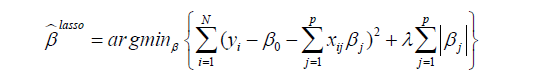
where y_i is the outcome and x_ij is the element of covariate vector. The subscript i represents the index of an observation and j is the index of a covariate. β₀ is the intercept term and β_j are coefficients to be estimated. It is noted that the first part of the equation is the regularization term and lambda is a free parameter which determines the amount of regularization. The term is a L1 Norm. In mathematics, the L1 Norm refers to the taxicab distance between two vectors:

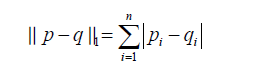
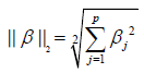
where p and q are vectors with n elements. It is noted that the L1 Norm is the sum of absolute difference. In contrast, the ridge regression employs L2 Norm that can be written as:

In our example, the coefficient of an interaction term can be shrunken to zero if there is no or minor interaction effect. Before running the LASSO variable selection procedure, we need to define model matrix to specify the model structure.

The model.matrix() function creates a model matrix by expanding factors into dummy variables and interactions. For example, the variable x2 is a factor and it is expanded to x21 to indicate level value 1 for x2 if x21=1, and 0 otherwise. The formula (x1+x2+t+x3+x4)³ is equivalent to (x1+x2+t+x3+x4)×(x1+x2+t+x3+x4)×(x1+x2+t+x3+x4) which in turn expands to a formula containing the main effects for x1, x2, x3, x4 and t together with their second and third-order interactions. The resulting matrix contains 26 terms including third-order interactions. The true significant interaction term (x1:x21:t) is also contained in the matrix. A downside of LASSO is that it assumes that all effects are linear and it does not search for split points.

The glmnet package (2.0-13) is employed for performing the LASSO regression. The above code firstly loads and attaches the glmnet package to the workspace, and then performs k-fold cross-validation for glmnet, produces a plot, and returns a value for lambda. The core to the feature variable selection is the cross-validation procedure, during which part of the data is used for fitting each competing model and the rest of the data is used to measure the predictive performances of the models by the validation errors, and the model with the best overall performance is selected. By default, the cv.glmnet() function uses 10-fold cross validation. The original sample is randomly split into 10 equal sized subsamples. One sample is used as validation data, and the remaining 9 of the 10 subsamples are used as training data. The cross-validation process is repeated for 10 times (the folds), with each of the 10 subsamples used exactly once as the validation data (8). Validation error of the fitted model is obtained from the training data. Since there are 10 values for the validation error, they are averaged to obtain a summary value. Validation error can be represented by different measures for binomial response variable. The argument type.measure specifies statistics used as the criteria for 10-fold cross validation. Four string values “deviance”, “mae”, “class” and “auc” are allowed for the argument, representing actual deviance, mean absolute error, misclassification error and area under the ROC curve (for two-class logistic regression only), respectively. In the present example, we used “auc” to measure the discrimination of logistic regression models.

The first argument x for cv.glmnet() function is a matrix with columns represent feature variables and their interaction terms, and rows represent observations. The argument y is the response variable. For family=“binomial”, as is the case in this example, y should be a factor with two levels. The LASSO method is specified by setting alpha=1. After fitting the model, the coefficients for each variables and interactions term can be viewed by the following code.

By setting s = “lambda.min”, the variables and interactions are selected at the minimum value of lambda. From the above output, it is noted that the coefficient for the term x1:x21:tA is 1.51. The changing pattern of AUC with different lambda values can be visualized.

Figure 1 is the cross-validation curve plotting AUC values against lambda values. Two selected lambda values which give the maximum AUC (minimum error) and the most regularized model such that error is within one standard error of the minimum, are indicated by two vertical dashed lines. The selected lambda values can be visited by the following code:

Figure 1 Cross-validation curve plotting AUC values against lambda values. The algorithm tries to find a parsimonious model with a large AUC value. Two selected lambda values which give the maximum AUC (minimum error) and the most regularized model such that error is within one standard error of the minimum, are indicated by two vertical dashed lines.

The LASSO model can be fit with the following code.

The glmnet() function fits a generalized linear model via penalized maximum likelihood. The regularization path is computed for the lasso penalty at a grid of values for the regularization parameter lambda. It is noted that the argument specification is the same as the one in the cv.glmnet() function.

The above code generates a coefficient path at different L1 Norm values (Figure 2). Each colored line represents the value taken by a different coefficient in the model.

Figure 2 Coefficient path at different L1 Norm values. The coefficients including interaction terms shrink with decreasing values of L1 Norm (more panelized). It is noteworthy that x1, x2 and x1:x2:t are the last terms shrunken to zero.

Lambda is the weight given to the regularization term (the L1 norm), so as lambda approaches zero, the loss function of the model approaches the ordinary least square (OLS) loss function. In other words, when lambda is very small, the LASSO solution should be very close to the OLS solution, and all of the coefficients are in the model. As lambda becomes larger, the effect of the regularization term increases and you will see fewer variables in the model (because more and more coefficients will be shrunken to zero).

As mentioned above, the L1 norm is the regularization term for LASSO. Another way to look at this is that the x-axis is the maximum permissible value the L1 norm can take. So when you have a small L1 norm, you have a lot of regularization. Therefore, an L1 norm of zero gives an empty model, and as you increase the L1 norm, variables will “enter” the model as their coefficients take non-zero values.

It is noteworthy that the interaction term x1:x21:tA is the last term to be shrunken to zero, indicating there is a subgroup defined by the variables x1 and x2.

Model-based recursive partitioning

Model-based recursive partitioning can be used to identify subgroups of patients with different responses to a given treatment. The approach incorporates recursive partitioning into conventional parametric model. At the beginning, a parametric model (e.g., logistic regression model) is fitted to the whole dataset. Then, parameter instability is tested over all potential splitting variables, and the parent node is split by a variable at a specific cutoff point which results in the highest parameter instability (9,10). The highest parameter instability is searched because we want to ensure the daughter nodes have the largest difference in model parameters. In our situation, the difference in parameter is equivalent to the difference in treatment effect size.

For treatment-subgroup identification this model contains the treatment as a covariate. In the case of a logistic regression model, for example, the model parameters are the intercept and the treatment effect. This model is the basis for the subgroup identification.

The current version of model4you package (version: 0.9-0) requires numeric variables for further analysis, thus the data frame is first transformed before fitting a base model. Then, the base model is computed for the given simulated data. The model-based recursive partitioning algorithm starts by computing the model for the entire dataset and tests for instability in the model parameters (e.g., intercept and treatment effect) by testing for independence between each patient characteristic and the partial score contributions. If instability is found, the patient characteristic corresponding to the test with the smallest P value is chosen as split variable and defines the subgroups. For each subgroup, the model is computed and again tested for parameter instability. This goes on until no further instability can be found or other stop criteria are fulfilled. Through this process the algorithm detects patient characteristics that have an effect on the outcome and/or interact with the treatment.

The pmtree() function in the model4you package is used to compute a model-based tree.

The pmtree() function takes the fitted base model (model4you package). Patient characteristics to be used for splitting can be set via the zformula argument (default is to use all remaining variables). Stopping criteria, such as the minimum number of observations per subgroup (minbucket), and other algorithm settings can be set via the control argument. The tree can be visualized as follows:

Figure 3 shows the visualization of the model-based tree. The tree recovers the data generating process quite well. It first splits in x1 close to zero (−0.006) and then in x2. Due to the linear effect of x1 on the outcome in the data generating process, the algorithm splits again in x1 for patients with x2=0 (see the changes in intercept). As for other model implementations in R, the summary() function can be used for the examination of more statistics.

Figure 3 Model-based tree by the pmtree() function. The tree recovers the data generating process quite well. It first splits in x1 close to zero (−0.006) and then in x2. Due to the linear effect of x1 on the outcome in the data generating process, the algorithm splits again in x1 for patients with x2 = 0 (see the changes in intercept).

It gives the coefficients in all leaf nodes of the tree. According to the data generating process, x1 should be included in the model as a linear effect. This can be achieved in two different ways: With a model-based tree including x1 as a covariate, which can be achieved via the glmtree() function in the partykit package (version: 1.2-0).

Figure 4 shows that the population is first split by x2 and then by x1. The two terminal nodes (4 and 5) are subgroups that have opposite treatment effects.

Figure 4 Model-based tree by the glmtree() function.

Alternatively, the model can be fit with a partially additive linear model tree (PALM tree) including x1 as a covariate with fixed parameter across subgroups (palmtree() function in package palmtree version: 0.9-0).

The functions glmtree() and palmtree() use different tests for parameter instability and use a different syntax for specifying the model (via the formula argument), but are closely related to pmtree(). The plots are shown in Figures 4,5. Of the three model-based trees, the palmtree() is the one representing the data generating process best, then glmtree(), and finally pmtree().

Figure 5 Model-based tree by the palmtree() function.

The QUINT method

The QUalitative INteraction Trees (QUINT) method, which was first introduced by Dusseldorp E and Mechelen IV, aims to subdivide the study population into subgroups by using recursive partitioning (11). The terminal nodes (leaves) are then assigned to one of three classes. Class 1: the treatment has beneficial effect; class 2: the treatment is harmful; class 3: the treatment and control groups have a similar effect. There are two components for the partitioning criteria: the difference in treatment outcome and the cardinality component. While the former ensures that the treatment difference in subgroups is sufficiently large, the latter ensures that the number of patients in a subgroup is sizable. The global partitioning criterion, denoted as C, is the combination of the two components. The goal of recursive partitioning is to maximize criterion C via an exhaustive search of all possible split variables and split points.

The QUINT method can be easily performed using the quint package (version: 1.2.1) (12).

The formula passed to the quint() function describes the model to be fit. The function requires a continuous outcome variable, thus the variable z is used instead of the binary variable y. In reality z would not be known, but the for the illustration purpose we used it here. The variable t before the “|” symbol is binary treatment variable, and variables after the “|” symbol are potential splitting variables.

The results are shown in Figure 6. At the top of the tree, the algorithm examines the parent node and looks for a feature variable at a cutoff point that can split the node into child nodes with increasing values in criterion C. Also, the child nodes can be assigned to one of the three classes as mentioned before. In the example, x1 is first chosen as a splitting variable at the cutoff value of 0. The binary splitting results in two child variables. The algorithm repeats the procedure until a split can no longer results in a higher value of C. The second split is based on x2. Since x2 is a factor variable with two levels, there is no need to find a cutoff point. The QUINT algorithm results in four leaves. The P1 leaf with green color represents the subgroup of patients who benefit from treatment. P2 represents the subgroup of patients for whom the treatment is harmful, and the P3 leaves represent the subgroup of patients for whom the treatment is neutral. The main results of the QUINT algorithm can be viewed with the summary() function.

The summary output contains fit, split and leaf information in sequence. The fit information shows the criterion C value for each split. It is noteworthy that the criterion C value increases from 2.73 to 3.70 when the tree is growing. The split information shows the split point for each variable. The leaf information table gives mean values of Y for the treatment and control groups in each leaf, as well as the mean difference (column d). The mean difference is also displayed in the leaves of Figure 6.

Figure 6 Partitioning tree based on the QUINT method. x1 is first chosen as a splitting variable at the cutoff value of 0. The binary splitting results in two child variables. The second split is based on x2. Since x2 is a factor variable with two levels, there is no need to find a cutoff point. The QUINT algorithm results in four leaves. The P1 leaf with green color represents the subgroup of patients who benefit from treatment. P2 represents the subgroup of patients for whom the treatment is harmful, and the P3 leaves represent the subgroup of patients for whom the treatment is neutral.

Adapted support vector machine classifier

Imai K and Ratkovic M proposed an adapted supporter vector machine classifier by placing separate sparsity constraints over the pretreatment parameters and causal heterogeneity parameters. In this framework, the conditional average treatment effect (CATE) can be estimated as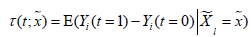, which can also be considered as the difference in predicted values under different treatment assignments conditional on covariates (13). The FindIt package is designed to estimate heterogeneous treatment effects, and it returns a model with the most predictive treatment-covariate interactions.

The binary outcome variable will be transformed by the formula in the package (13). To make sure the outcome variable takes the value of 1 or -1, the outcome y in the original data need to be transformed to take values 0 and 1. In our example, the variable y is a factor which would be transformed into a numeric variable with values 1 and 2 by the as.numeric() function. Thus, we need to minus 1 from the transformed numeric values.

The above code specifies the model structure. The model.treat argument specifies the outcome and treatment variables. model.main specifies pre-treatment covariates to be adjusted for, and model.int specifies pre-treatment covariates to be interacted with treatment variable when treat.type=“single”. The type argument receives a string “binary” to indicate that the outcome variable is a binary outcome. A “single” treatment type indicates interactions between a single treatment variable.

The predict() function is employed to estimate the treatment effect of each individual patient. The output shows 10 patients with the most positive treatment effect and 10 patients with the most negative treatment effect. It appears that patients with positive treatment effect have x1>0 and x2=1, whereas patients with negative treatment effect have x1<0 and x2=1. The results can be visualized with the following code. While the treatment effect is not precisely a difference in probabilities, the algorithm approximates probabilistic estimates of the CATE.

The output is shown in Figure 7, plotting treatment effect against index of observation. The treatment effects are heterogeneous in the study population with subgroups for whom the treatment can be beneficial or harmful. We can also examine the distribution of treatment effects in the x1*x2 covariate space with contour plot.

The colorRampPalette() function returns functions that interpolate a set of given colors to create new color palettes. In the example, three colors “red”, “yellow” and “green” are mixed to generate a new color palette. The contour plot shows that the subgroups for whom the treatment is beneficial and harmful represented by green and red colors, respectively, are defined by x1 at cutoff point of 0 and x2 (Figure 8).

Figure 7 Heterogeneous treatment effect across the study population. Treatment effect is plotted against index of observation.

Figure 8 Contour plot showing the distribution of treatment effects in covariate spaces defined by x1 and x2. It is noted that the subgroups in which the treatment is beneficial and harmful effects as represented by green and red colors, respectively, are by x1 at cutoff point of 0 and x2.

Virtual twins method

The “virtual twins” method for the identification of subgroups of patients in RCTs has been previously described by Foster JC and colleagues (14). This method utilizes random forest ensemble to predict the probability of the outcome of interest for each subject in a counterfactual framework. Thus, there are two response probabilities, representing the treatment and control “twins”, for each patient. The difference in probabilities of the event of interest for the treatment and control “twins” is estimated as Z_i = P_1i –P_0i, which can be considered as treatment effect for patient i. Then a regression or classification tree is built by including Z_i as response variable, and other baseline feature variables as the covariates (15). The aim of the method is to identify a set of covariates Xs which are strongly associated with Z and thereafter to define a region A in which the treatment effect is significantly better than the average effect. The virtual twins algorithm can be performed using the aVirtualTwins package in R.

The formatRCTDataset() function generates a dataset that can be analyzed using the Virtual Twins method. The dataset argument of the function is a typical data frame recording RCT data. The outcome and treatment variables should be explicitly defined by “y” and “t”, respectively.

The vt.data() function is a wrapper of formatRCTDataset() and VT.objectm to initialize Virtual Twins data. The argument of the function is similar to the formatRCTDataset() function.

The above code creates a random forest to compute the difference in treatment and control “twins” (Z_i). By default, the difference is measured in absolute scale: Z_i = P_1i – P_0i. Other scales for the difference include “relative” (P_1i /P_0i) and “logit” (logit(P_1i) – logit(P_0i), which can be specified in the vt.forest() function by method=c("absolute", "relative", "logit"). The resulting difference can be visited in the object vt.f$difft. As shown in the above output, the difference in absolute scale ranges from -0.58 to 0.67.

The difference computed by random forest can be visualized with contour plot (Figure 9). It is noteworthy that the difference Z is well separated by the x1*x2 covariate space.

Figure 9 The distribution of the difference in probabilities of the event of interest for the treatment and control “twins”. It is noted that the subgroups in which the treatment is beneficial and harmful effects as represented by green and red colors, respectively, are by x1 at cutoff point of 0 and x2.

The vt.tree() function tries to find a strong association between difference Z and covariates (e.g., which covariates are associated with big change in Z). When setting tree.type=“class”, a classification tree is fitted by creating a new variable Z* = 1 if Z_i > c and Z* = 0 if Z_i ≤ c. In the example, the threshold for classification regression is set at 0.01. The new binary variable Z* is used as the outcome in fitting the classification tree. By setting tree.type=“reg”, a regression tree is computed on Z, with covariates X. The regression tree is then used to predict Z_i value for each patient. Then patients with predicted Z_i greater than a threshold value are categorized into region A. In the example, the threshold is set at 0.1. The regression and classification tree can be visualized using the rpart.plot() function.

The results are shown in Figure 10. The upper plot shows the classification tree. The package employs rpart() function to perform tree modeling, in which the Gini index is used to measure the impurity in each node (16). By setting extra=102, the classification rate, expressed as the number of correct classifications and the number of observations, is displayed in each node. The root node is split by x1 at the value of 0.035. If x1<0.035, the tree predicts patients belonging to the class with Z* =0, which is not the class of interest in the example (e.g., recall that the algorithm tries to find a region A where the difference in treatment effect is greater than c=0.01. Z_i ≤ c in the region defined by x<0.035). In contrast, the covariate space x1≥0.035 and x2≥0.5 defines a region where Z_i>c. It is noteworthy that 281 of the 288 patients at the rightmost terminal node have Z*=1, which is the exact region the vt.tree() function tries to find. Also note that x2 has been transformed to a numeric variable and its cutoff value is 0.5, instead of the binary value 0 and 1. The regression tree shows the difference in probability Z_i at inner and terminal nodes. The percentage of patients is shown at the bottom of each node. In the terminal node defined by x1≥0.047 and x2≥0.5, the difference in probabilities of the treatment and control “twins” is 0.23, which accounts for 14% of the whole study population.

Figure 10 Classification (upper panel) and regression (bottom panel) trees partitioning the whole study population into subgroups. The subgroup in which the difference in probabilities is greater than a prespecified value c is of interest. The classification tree (upper panel) predicts patients belong to the class with Z* = 0 when x<0.035, which is not the class of interest in the example. In contrast, the covariate space x1≥0.035 and x2≥0.5 defines a region where Z_i > c. It is noteworthy that 281 of the 288 patients at the rightmost terminal node have Z* = 1, which is the exact region the vt.tree() function tries to find. The regression tree (bottom panel) shows the difference in probability Z_i at inner and terminal nodes. The percentage of patients are shown at the bottom of each nodes. In the terminal node defined by x1≥ 0.047 and x2≥0.5, the difference in probabilities of the treatment and control “twins” is 0.23, which accounts for 14% of the whole study population.

Summary

This article reviews several commonly used methods for the identification of subgroups. Simple regression based methods are generally easy to understand and can be implemented by most clinical investigators. However, such methods require hypothesis on interaction terms and higher-order interactions are often missed. Panelized regression model is able to search a large number of covariate and interaction terms, shrinking unimportant terms. However, the selection of penalty value is somewhat arbitrary. Model-based regression tree has more direct interpretation than higher-order interaction terms but they have inherent limitations of identifying subgroups that cannot be verified in subsequent trials (e.g., false positive results). Furthermore, the parameter confidence interval is questionable (9,17). The QUINT method reported qualitative treatment-subgroup interactions and is suitable for studies aiming to assign patients to optimal treatments. Virtual Twins method works in a counterfactual framework and treatment effects of each subject can be estimated. In conclusion, all methods have their limitations and advantages. No one is definitively superior to the other and the choice on which to use depends on the specific questions under investigation, as well as the familiarity of the investigators to a specific method (Table 1).

Table 1 Comparisons of different methods for subgroup identification
Full table

Acknowledgements

Funding: Z Zhang was supported by Zhejiang Provincial Natural Science foundation of China (LGF18H150005).

Footnote

Conflicts of Interest: The authors have no conflicts of interest to declare.

References

1. Nallamothu BK, Hayward RA, Bates ER. Beyond the randomized clinical trial: the role of effectiveness studies in evaluating cardiovascular therapies. Circulation 2008;118:1294-303. [Crossref] [PubMed]
2. Oude Rengerink K, Kalkman S, Collier S, et al. Series: Pragmatic trials and real world evidence: Paper 3. Patient selection challenges and consequences. J Clin Epidemiol 2017;89:173-80. [Crossref] [PubMed]
3. Lipkovich I, Dmitrienko A, D'Agostino B R Sr. Tutorial in biostatistics: data-driven subgroup identification and analysis in clinical trials. Stat Med 2017;36:136-96. [Crossref] [PubMed]
4. Kehl V, Ulm K. Responder identification in clinical trials with censored data. Computational Statistics & Data Analysis 2006;50:1338-55. [Crossref]
5. Pavlou M, Ambler G, Seaman S, et al. Review and evaluation of penalised regression methods for risk prediction in low-dimensional data with few events. Stat Med 2016;35:1159-77. [Crossref] [PubMed]
6. Tibshirani R. Regression shrinkage and selection via the lasso: A retrospective. J R Statist Soc B 2011;73:273-82. [Crossref]
7. Hastie T, Friedman J, Tibshirani R. Linear Methods for Regression. In: Hastie T, Tibshirani R, Friedman J. editors. The Elements of Statistical Learning. 2nd ed. New York, NY: Springer New York, 2009:43-100.
8. Jung Y, Hu J. A K-fold Averaging Cross-validation Procedure. J Nonparametr Stat 2015;27:167-79. [Crossref] [PubMed]
9. Seibold H, Zeileis A, Hothorn T. Model-Based Recursive Partitioning for Subgroup Analyses. Int J Biostat 2016;12:45-63. [Crossref] [PubMed]
10. Zeileis A, Hothorn T, Hornik K. Model-Based Recursive Partitioning. J Comput Graph Stat 2008;17:492-514. [Crossref]
11. Dusseldorp E, Van Mechelen I. Qualitative interaction trees: a tool to identify qualitative treatment-subgroup interactions. Stat Med 2014;33:219-37. [Crossref] [PubMed]
12. Dusseldorp E, Doove L, Mechelen Iv. Quint: An R package for the identification of subgroups of clients who differ in which treatment alternative is best for them. Behav Res Methods 2016;48:650-63. [Crossref] [PubMed]
13. Imai K, Ratkovic M. Estimating treatment effect heterogeneity in randomized program evaluation. Ann Appl Stat 2013;7:443-70. [Crossref]
14. Foster JC, Taylor JM, Ruberg SJ. Subgroup identification from randomized clinical trial data. Stat Med 2011;30:2867-80. [Crossref] [PubMed]
15. Loh WY. Classification and regression trees. Wiley Interdiscip Rev Data Min Knowl Discov 2011;1:14-23. [Crossref]
16. Merkle EC, Shaffer VA. Binary recursive partitioning: background, methods, and application to psychology. Br J Math Stat Psychol 2011;64:161-81. [Crossref] [PubMed]
17. Leeb H, Pötscher BM. Model selection and inference: Facts and fiction. Econometric Theory 2005;21:21-59. [Crossref]