Overview of model validation for survival regression model with competing risks using melanoma study data
Introduction
Model validation plays an important role in identifying the problem of model misspecification and overfitting. A model is considered to be overfitted if it has a good prediction accuracy in a training dataset but a poor prediction accuracy in a testing dataset. In such a circumstance, one may need to revisit the specification of the model (i.e., the proportionality assumption, interaction, and variable selection). Multi-state and competing risks are settings where, in addition to the main survival time endpoint, the cause (or type) of failure and other intermediate events are also observed during the follow-up time period. In the competing risks model, two or more causes of failures can act simultaneously, but only the earlier failure and its cause are observed. The competing risks analysis is a special case of the survival analysis when an individual experiences one of several different types of events. The occurrence of competing events prevents the occurrence of an event of interest (1), and vice versa. For example, researchers may be interested in cancer-specific death, but some patients may die of other causes irrelevant to cancer prior to death from cancer, yielding two competing causes of death. The event of interest is death from cancer, but the occurrence of death from other causes prevents the occurrence of death from cancer.
In a standard Cox regression model, competing events may be regarded as non-informative censoring, that is, their occurrence has no impact on subsequent occurrence of the event of interest. In fact, this is the typical case in many practical data applications. In competing risks analysis the main quantity of interest is typically the cumulative incidence function of a certain type of event in a specific time period [0,t], which represent the cumulative risk of experiencing this type of event before or at time t, given the presence of the remaining competing events.
In the literature there exists several regression approaches to modelling competing risks data, and they have the potential to respond to different research questions. The first approach, generally mentioned as “cause-specific hazards” approach, models the cumulative incidence via all the cause-specific hazards (2,3). A second approach is the Fine-Gray model (4), where the cumulative incidence is estimated via the sub-distribution hazard.
In a previous article (5), we have reviewed methods on how to draw nomogram for survival model in the presence of competing risks. In this paper, we review methods for validating competing risks regression models and provide R code for implementing model validation with a detailed explanation.
Working example
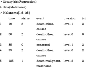
We illustrate how to validate competing risks regression models using Melanoma dataset included in the riskRegression package (6). The dataset contains a cohort of 205 patients with melanoma. By the end of follow-up, there are 134 survivors and 71 non-survivors. The time is the days after operation, and status is vital status (0= censored, 1= death due to melanoma and 2= death due to other causes), where death from melanoma is an event of interest and death from other causes is a competing event. There are seven predictors measured at the start of follow-up: age, sex, tumor thickness (thick), ulcer, invasion, inflammatory cell infiltration (ici) and epicel. The first five patients can be viewed using the following code:
As shown in the above table, the first patient died due to other causes at 10 days after operation. She has level 1 invasion and grade 2 inflammatory cell infiltration.
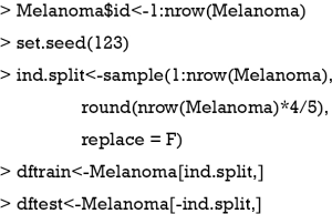
The above code generates a new variable id to indicate unique identification number for each patient. The dataset is randomly split into training (80%) and testing (20%) datasets.
Cause-specific hazard model versus Fine-Gray model
In the regression analysis of competing risks data, the effects of covariates on the cause-specific hazard function or cumulative incidence function can be investigated via the cause-specific hazards model or Fine-Gray (subdistribution hazard) model, respectively. In the cause-specific hazards model, a hazard ratio represents the instantaneous relative risk of an event of interest in the presence of the covariate (e.g., the ratio of the hazard rates corresponding to the conditions described by two different levels of an explanatory variable, all other covariates being equal). However, this hazard ratio cannot be directly translated to the cumulative incidence function which is clinically relevant and may provide useful information to researchers. The Fine-Gray model addresses this issue and has the advantage that the cumulative incidence of the event of interest has a direct link with the estimated sub-distribution hazard, and thus regression coefficients quantify the direct effects of covariates on the cumulative incidence. However, the estimated sub-distribution hazard ratio from Fine-Gray model has no direct clinical interpretation because the survival times of subjects who did not experience the event of interest are transformed into censored times that are artificially extended to infinity. Moreover, the probabilistic relationship between the cumulative incidences of the different types of events and the marginal survival function is lost.
Finally, for the above reason, these two models are recommended to be reported simultaneously in the analysis of competing risks (7).
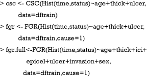
The R function Hist() is similar to the Surv() function in the survival package, which provides functionality for managing censored event history response data. In the example, the time and status are numeric vectors used for specifying the observed time and vital status, respectively. The CSC() function is used to fit the cause-specific proportional hazards model, where the first vital status is used as a cause of interest by default. Alternatively, the cause argument can be used to specify a cause of interest. FGR() is an interface for fitting the Fine-Gray model and the arguments of the function are similar to that of the CSC() function. A full model (fgr.full) is fitted by using the Fine-Gray model including all seven predictors. Predictions based on these fitted models can be obtained using the following code, which provides predictions of the cumulative incidence functions for death from melanoma for the first five individuals in the test dataset over 1,000 to 4,000 days after operation. The absolute risk of each individual can be obtained by using the autoplot() function.
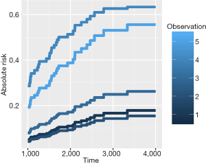
Figure 1 shows the cumulative incidence estimates (i.e., absolute risk) for death from melanoma for each of the five individuals. It appears that patient #4 has the highest melanoma mortality rate over the entire follow-up period. The absolute risk of each individual can be obtained by using the following code:
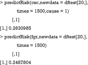
The predict() and predictRisk() function are similar that both of them estimate the absolute risk at specified time points. The difference is that the former returns covariates that have been used for prediction, whereas the latter only reports the absolute risk.
For patient #20, the cumulative incidence estimates by 1,500 days for death from melanoma are 0.26 under the cause-specific proportional hazards model and 0.25 under the Fine-Gray model. The difference between estimates of the cumulative incidence function from a Fine-Gray model and from cause-specific hazards models is caused by different proportionality assumptions—proportional subdistribution hazards for the Fine-Gray model and proportional cause-specific hazard for both Cox regression models.
Calibration plot
A calibration plot is used to compare the predicted probability with the observed probability at a certain time point. If a model is ideal, pairs of the observed and predicted probabilities lie on the 45-degree angle line, implying that both probabilities match well to each other.
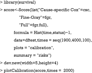
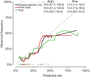
The Score() function provides a set of methods to score the predictive performance of risk prediction models. The first argument is an object or a list of objects of risk prediction models. In the example, all three models were assessed for their predictive performance. The data argument specifies a dataset that will be used for predictions. Recall that we split Melanoma data into the training and test datasets. The former is used to train a model, and the latter is used to assess model fit. The times argument specifies a series of horizons for prediction. The plot argument defines a plot to be drawn and corresponding data suitable for the plot are put into the results. Finally, the plotCalibration() function draws a calibration plot (Figure 2). The closer of a calibration curve of a model to the diagonal, the better of the model. Furthermore, the area under operating characteristic curve (AUC) and Brier score are shown at the top of Figure 2. The AUC, also known as C-index, is used to assess the discrimination of a model (8). If the AUC >0.8, it indicates that the discriminatory accuracy of a model is good. The Brier score measures discrimination and calibration at the same time (9). The Brier score for an event of interest at a time is defined as the expected squared distance between the observed status at that time and the predicted probability. Thus, a smaller value of Brier score indicates a better model. In our example, the full model has the smallest AUC and the largest Brier score.
Calibration with cross validation method
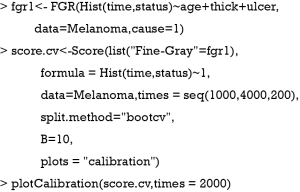
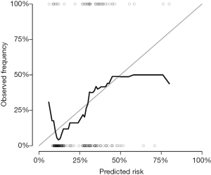
The above example split the dataset into training and test datasets once. This could be problematic since the test set we used can happen to be particularly easy (or hard) to predict. Thus, it is necessary to use all the data for both model training and validation. That is the reason why we use the cross-validation method (10). A commonly used cross-validation method is the k-fold cross-validation, which has been also applied to competing risks regression models (11,12). The original sample is randomly partitioned into k equal sized subsamples. Of the k subsamples, a single subsample is retained as the validation data for testing a model, and the remaining k−1 subsamples are used as training data. The cross-validation process is then repeated k times, with each of the k subsamples used exactly once as the validation data. The k results can then be averaged to produce a single estimation. The prediction accuracy index can be AUC or Brier score in our example. However, unlike the one-time splitting method, the cross validation will result in k models, and the next question goes to which one should be the best to use for prediction. The answer is that the purpose of cross-validation is not to come up with a final model, but it consists only of model checking for improving prediction accuracy. We do not use these k instances of our trained model to do any real prediction. To reach this scope, we want to use all available data to come up with the best possible model. The purpose of cross-validation is model checking, not model building. We can compare model specification by using cross-validation. Suppose we have linear regression models with and without interaction, cross-validation methods can suggest which model is better in terms of prediction, and then we can train that model using all data. Note that although the covariate effects in the linear model can be different for each training iteration, the model specification is the same across these iterations. Alternatively, we can use cross-validation to build an ensemble model.
Figure 3 shows the calibration plots for Fine-Gray model at day 2,000. Note that the whole dataset is used in fitting the model.
Bandwidth selection
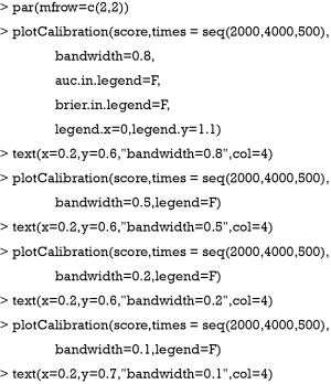
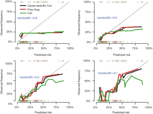
A smother calibration curve can be obtained by different smoothing methods, which however rely on the choice of a bandwidth (6). The shape of a calibration curve largely depends on the choice of bandwidth. A large bandwidth may result in a smooth and flat curve (large bias but small variance), but a small bandwidth will result in wiggly curve (small bias but large variance). Thus, the choice of bandwidth is a trade-off between the bias and variance. The following code generates calibration curves with different bandwidths.
At a bandwidth of 0.8, nearly all observations are grouped as one risk group, thus the calibration curves are identical for all three models and are flat and smooth. In contrast, the curves with bandwidth =0.1 appear to be wiggly (Figure 4).
Plotting AUC and Brier score over follow-up time
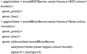
The above example shows the calibration and discrimination at a specific time point, which is not the whole picture for entire period under study. Researchers may also be interested in the prediction accuracy of a model over entire follow up time period. Fortunately, the Score() function calculates all these scores over time and users can easily extract the results for further graphical display. Here, we use ggplot2 package for drawing plots (13).
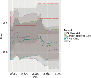
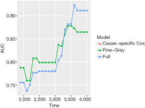
The object score returned by the Score() function is a list containing a variety of objects. The structure of this list can be viewed by the str(score) syntax. The AUCs of all models across all times can be extracted by score$AUC$score. The geom_ribbon() is a layer added to the ggplot object. The Brier score can be plotted over time in the same way. Figure 5 shows the AUC for all three models. Note that the cause-specific hazard model has the same values to that of the Fine-Gray model, and their dots and lines overlap. Also note that the models have higher discriminatory accuracy at later follow-up times. Figure 6 shows the Brier score for all models (e.g., null, cause-specific, Fine-Gray and full models).
Nomogram for visualizing regression models
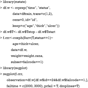
The regplot() function provides tools for plotting nomograms with good aesthetics. However, it receives only objects returned by coxph, lm and glm. Thus, in order to draw a nomogram in the presence of competing risks, we need to create weighted data set for competing risks analyses (14), as explained in the following R code. In this way, the competing risk model can be fitted with the coxph() function and then passed to the regplot() to draw a nomogram.
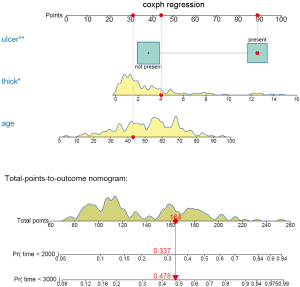
The above code firstly creates a weighted data set, and then the competing risk analysis with Fine-Gray model is performed with the coxph() function. Finally, the regplot() is employed to depict a nomogram. The patient #24 is illustrated in the nomogram by mapping its values to the covariate scales. The cumulative incidence estimates for death from melanoma by day 2,000 and 3,000 are 0.33 and 0.473, respectively (Figure 7).
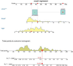
The probability is 0.478 at time 3,000 in the cause-specific hazard model (Figure 8), which is slightly higher than the estimate under Fine-Gray model.
Discussion
This article reviewed methods for validating competing risks regression models. The original sample is split randomly into training and test datasets. However, this one-time splitting method reduces sample size of both model training and test datasets. Roecker stated that “(this method) appears to be a costly approach, both in terms of predictive accuracy of the fitted model and the precision of our estimate of the accuracy.” (15) Furthermore, the accuracy can be fortuitous that different processes may result in different estimates. The cross-validation method is more appealing in this aspect and has been more widely used. It should be noted that the cross-validation method aims to validate a model, not to build a model. Thus, the final model can be derived by fitting a model on the whole dataset after cross-validation. The cross-validation tells you how to specify a model (e.g., variable selection, transformation and interaction). The prediction accuracy of the fitted model can be assessed by discrimination and calibration. The former is represented by the AUC or C-index; and the latter can be assessed by inspecting a calibration plot. The Brier score takes into account the discrimination and calibration at the same time. Finally, nomograms can be used to visualize a trained model. Since the regplot() function cannot process object returned by FGR() function, the competing risk model have to be fitted by using coxph() with a weighted dataset.
Acknowledgements
Funding: Z Zhang received funding from the Public Welfare Research Project of Zhejiang province (No. LGF18H150005) and Scientific Research Project of Zhejiang Education Commission (No. Y201737841); M Lee received a grant from Basic Science Research Program through the National Research Foundation of Korea (NRF) funded by the Ministry of Education (No. NRF-2018R1D1A1B07041070).
Footnote
Conflicts of Interest: The authors have no conflicts of interest to declare.
References
- Putter H, Fiocco M, Geskus RB. Tutorial in biostatistics: competing risks and multi-state models. Stat Med 2007;26:2389-430. [Crossref] [PubMed]
- Prentice RL, Kalbfleisch JD, Peterson AV Jr, et al. The analysis of failure times in the presence of competing risks. Biometrics 1978;34:541-54. [Crossref] [PubMed]
- Cox DR. Regression Models and Life-Tables. J R Stat Soc Series B Stat Methodol 1972;34:187-220.
- Fine JP, Gray RJ. A Proportional Hazards Model for the Subdistribution of a Competing Risk. J Am Stat Assoc 1999;94:496-509. [Crossref]
- Zhang Z, Geskus RB, Kattan MW, et al. Nomogram for survival analysis in the presence of competing risks. Ann Transl Med 2017;5:403. [Crossref] [PubMed]
- Gerds TA, Ozenne B. riskRegression: Risk Regression Models and Prediction Scores for Survival Analysis with Competing Risks. 2018. Available online: https://CRAN.R-project.org/package=riskRegression
- Latouche A, Allignol A, Beyersmann J, et al. A competing risks analysis should report results on all cause-specific hazards and cumulative incidence functions. J Clin Epidemiol 2013;66:648-53. [Crossref] [PubMed]
- Schoop R, Beyersmann J, Schumacher M, et al. Quantifying the predictive accuracy of time-to-event models in the presence of competing risks. Biom J 2011;53:88-112. [Crossref] [PubMed]
- Gerds TA, Andersen PK, Kattan MW. Calibration plots for risk prediction models in the presence of competing risks. Stat Med 2014;33:3191-203. [Crossref] [PubMed]
- Harrell FE. Regression Modeling Strategies. New York, NY: Springer New York, 2001.
- Lee M, Cronin KA, Gail MH, et al. Predicting the absolute risk of dying from colorectal cancer and from other causes using population-based cancer registry data. Stat Med 2012;31:489-500. [Crossref] [PubMed]
- Cortese G, Gerds TA, Andersen PK. Comparing predictions among competing risks models with time-dependent covariates. Stat Med 2013;32:3089-101. [Crossref] [PubMed]
- Wickham H. ggplot2: Elegant Graphics for Data Analysis. Springer International Publishing, 2016.
- Geskus RB. Cause-specific cumulative incidence estimation and the fine and gray model under both left truncation and right censoring. Biometrics 2011;67:39-49. [Crossref] [PubMed]
- Roecker EB. Prediction Error and Its Estimation for Subset-Selected Models. Technometrics 1991;33:459-68. [Crossref]

