Propensity score analysis for time-dependent exposure
Introduction
Propensity score analysis (PSA) is widely used in medical literature. In observational studies, the causal inference cannot be easily made due to multiple measured and/or unmeasured confounding factors. The causation between exposure (A) and outcome (Y) is explored in counterfactual framework so that the allocation of treatment (i.e., the treatment a subject actually receives) is independent of potential outcome Ya conditional on confounders (L) such as the severity of illness and patients’ preference: . The treatment effect can then be estimated in the strata with equal probability of receiving treatment. Here comes the idea of propensity score (PS) which is typically estimated by regressing the treatment on pre-treatment covariates using binary logistic regression models. After PS matching, the matched cohort is considered as that generated from randomized experiments in which the treatment allocation is independent of any pre-treatment covariates.
However, PS is generated for each individual at study entry without considering its time-dependent property. In effect, there are many interventions that are not given at the start of a study but may be given at any time during study period. For example, in a study exploring the association of tracheal intubation and survival in in-hospital cardiac arrest, the tracheal intubation (exposure) can happen at any time after cardiac arrest and intubation may not occur if return of spontaneous circulation (ROSC) or termination of efforts occurs first (1). If the duration of resuscitation is long enough, a patient is very likely to be intubated. Thus, the comparison between intubated and non-intubated subjects is essentially comparing the survival outcome for those with long versus short resuscitation time. Short resuscitation time can be the result of early ROSC or termination of efforts. To avoid such bias, time-dependent PS matching can be performed by iteratively matching the treated subjects to the “at-risk” controls across all time strata.
This article aims to provide a step-by-step tutorial on how to perform analysis for time-dependent treatment. We will show how the conventional PSA ignoring the time-to-exposure property of the treatment can bias the result, and then highlight the time-dependent PS matching for the analysis of such data. Specifically, we provide a function TDPSM() to perform time-dependent PS matching. Alternative methods such as Cox regression with time-varying covariate, adjustment with PS are also shown for comparison. Comparisons among these methods are performed by simulation. Finally, we illustrate how to use the TDPSM() in real world data.
Working example
Mathematics underlying survival data simulation
We need to spend a little time to review mathematics underlying the survival analysis. Assume that the survival time T follows an exponential distribution, the baseline cumulative density function can be written as , where λ is a constant term. The function behaves reasonably that when t tends to 0, F0(t) tends to 0, as it should be (e.g., the cumulative probability of the event is small). When t tends to infinity, F0(t) tends to 1 (e.g., the event will eventually happen). Following this assumption, other important functions can be easily derived. The probability density function f0(t) is the first order derivative of the F0(t) w.r.t. t: f0(t) = F0'(t)= λe−λt. The survivor function is S0(t) = 1−F0(t)=e−λt; and the hazard function , which is a constant hazard. The cumulative hazard function is H0(t) = λt. The above equations define as the baseline function that all covariates are zero. The hazard function in the presence of covariates can be expressed as h(t) = λeβx. Since h(t) = λeβx is independent of t,. The survival time can be simulated by , where U follows a uniform distribution on the interval from 0 to 1, which is consistent with the survivor function S(t) (2). Simulation of longitudinal data with time dependent exposure is well described in Xu’s article (3). We adapted their approach as follows:
Next, we are going to simulate a dataset with time-varying exposure and survival outcome.
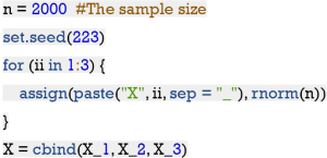
(I) Generate three confounders with standard normal distribution.
The sample size is 2000 and we also set a seed for reproducibility. In the for loop, three covariates X_1, X_2 and X_3 are generated.
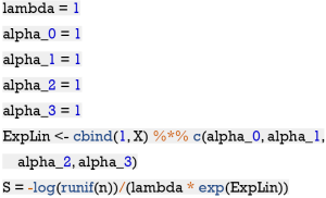
(II) Generate the potential exposure time S given X1, X2 and X3 from an exponential distribution with rate , where (a0,a1,a2,a3) =(1,1,1,1), and .
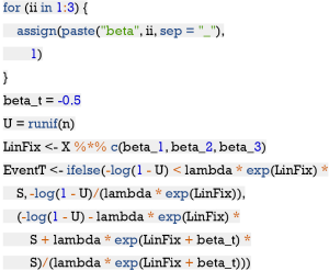
(III) Generate the event time T given X_1,X_2,X_3 and Z1(t) = I(t > S), where I(·) is the indicator function, according to a Cox model with hazard function
|
| [1] |
where h0(t) =1, β takes on the value of −0.5, and(β1,β2,β3) =(1,1,1). For the ease of annotation, we can write β'X = β1X1 + β2X2 + β3X3 as the linear predictor of time-fixed covariates The integration of h(t) w.r.t. t gives the cumulative hazard function
|
| [2] |
This gives the survival function
|
| [3] |
By sampling X and u~U(0,1), substituting u for S(t) and rearranging with simple algebra gives the following equation for T. (4)
|
| [4] |
where β'X = β1X1 + β2X2 + β3X3, and u~U(0,1). This is effectively a piecewise exponential distribution, with different rates on the two intervals (0,S) and (S,∞). The above mathematical equations can be coded as follows:
(IV) Generate censoring time CensorT as Uniform (0,b), where b =0.8 is chosen so that a pre-specified percentage of censoring is achieved. Then all simulated variables are merged into a data frame.
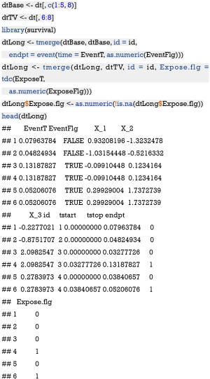
The dt is the prototype of a data set for survival analysis with time-dependent exposure. EventT is the observed time until censoring or the event of interest (i.e., mortality, recurrence and development of complications) occurs. EventFlg is whether a subject is right censored FALSE or event occurs TRUE. X_1 to X_3 are time-fixed covariates. ExposeFlg is exposure status and ExposeT is the time on which a subject is exposed. Note that the time-dependent exposure is a stochastic process (counting process) that equals zero from t0 until exposure, then it equals to one until the end of observation.
Alternative method to generate a data frame with counting process
Another way to generate simulated dataset with time-dependent exposure is to loop through individual subjects. We adapt code used in the genTDCM() function in the genSurv package (5,6).
The generated data is the same as dt, except that dt is not expanded. The variable tdcov corresponds to the ExposeFlg. In the next chunk, we are going to expand the dt with the tmerge() function so that each subject can have multiple intervals and thus takes multiple rows.
Effect estimates using Cox regression model with time-varying exposure
Because the exposure in the example is time-varying, i.e., subjects can receive treatment at different observation period, the treatment effect can be estimated by using the coxph() function (7). The following chunk first splits the variables into those that are time-varying (dtTV) or time-fixed (dtBase), and then generate the counting process table with tmerge() function.
The reformatted data frame is the same as the data generated above, with tstart and tstop corresponding to the start and stop variables in the data, respectively. Next, we will fit a Cox model with time-varying exposure.
The estimated treatment effect is −0.42 (P<0.001), which has little biased, and importantly the corresponding confidence interval includes the true effect of −0.5.
PSA by considering exposure as a binary variable
Conventionally, patients are simply divided into those exposed and non-exposed groups without considering the time-to-exposure property. In this scenario, PS can be generated by regressing the exposure status Z1(t) on baseline covariates X. Here we define the as a linear combination of covariates, which is monotone function of the probability of treatment exposure. Finally, the treatment effect can be estimated by adjusting for this PS1.
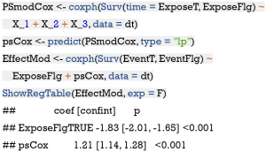
The estimated coefficient for the exposure is −1.83 (95% CI: −2.02 to −1.65), which is significantly downward biased comparing to the true effect of −0.5. PS can be used to match subjects with similar probability of receiving treatment exposure (8,9). Let’s see how the estimated treatment effect differs from the true one when the time-to-exposure is ignored. Here we use the MatchIt package to perform PS matching (10).
The results show that the estimated treatment effect is slightly upward biased comparing to the true effect.
PS generated by Cox regression model
In this instance, the PS is estimated by regressing the time to exposure on X with Cox regression model. The Cox regression model gives estimated coefficients, , , and . Here we define as a linear combination of covariates with estimated coefficients obtained from the Cox regression model. Strictly speaking, the PS2 cannot be called a PS because PS should be the probability of receiving treatment given covariates. PS2 is a surrogate for PS. The Cox regression model concerns the time-to-exposure feature in the estimation of PS2. Then the treatment effect is estimated in multivariate model by adjusting for the PS2.
The results show that the coefficient for the exposure is −1.83, which is an underestimation of the true treatment effect. The reason is probably that adjusting for PS2 directly in the outcome model is subject to model misspecification and thus fail to recover true effects. This lead us to consider PS matching, a non-parametric technique to reduce model dependence (8,10).
Time-dependent PS matching
The PS is estimated by Cox proportional hazard regression model, regressing time-to-exposure on time-fixed and time-varying covariates (e.g., only time-fixed covariates Xs are available in our example). Then the matching can be performed by sequential matching or simultaneous matching (11). Here we implement the sequential matching algorithm. The sequential matching takes place within risk set Rt at time t; Rt consists of all patients at risk of exposure at t. The matching procedure proceeds chronologically for each of the risk sets. There can be several subjects being treated at each risk set, and these patients compete with each other for matching controls. Note that the at-risk subjects being matched include those who are not exposed before or within the time interval t, and thus they also include those who are exposed latter. Remember that the matching should not depend on future data. The optimal matching can be easily performed by using the optmatch package (12). Then, matched individual subjects are removed from later risk sets Rt+1,t+2,.., and the process continues with the next risk set Rt+1 (11).
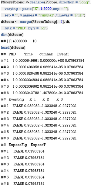
The above code chunk regresses the time to exposure on covariates Xs and estimates cumulative hazard for each individual over all time points that are experienced by sample patients. The survfit() function generates values for creating survival curves from previously fitted Cox model PSmodCox (13). Thus, the resulting PScore has the dimension of 2,000×2,001 with rows and columns corresponding to the time points and individual subjects, respectively. The values in the matrix are cumulative hazards. Next, let’s reshape the matrix for further matching.
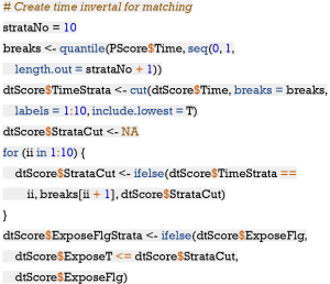
The reshape() function is employed to convert wide to long format (14). Then the long format data frame is merged with the original data frame dt. The resulting dtScore has 4,000,000×7 dimension. The matching procedure have to proceed at a specified time interval; thus the entire follow up time is divided into 10 equally spaced intervals (e.g., each interval contains equal number of subjects). We create a new variable TimeStrata to store the information.
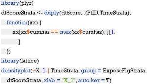
The dtScore must be formatted for matching procedure. Each individual subject has 2,000 rows with each representing a unique follow up time point. We only need to keep one row with the maximum cumulative hazard for each combination of PtID and TimeStrata, which can be easily performed by using the ddply() function.
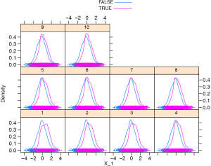
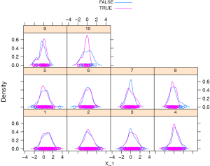
The density plot shows that the distribution of X_1 is different between the treated and the controls (Figure 1). Let’s see how to match them (i.e., select control subjects with similar cumulative hazard to the treated in each risk set) with sequential matching.
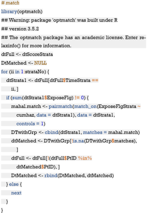
The sequential matching proceeds iteratively from TimeStrata = 1 to 10, thus we used a for loop to perform the task. Each TimeStrata is considered as a risk set, within which the exposed subjects is matched to the controls. Recall that we have estimated cumulative hazard for the controls at each time strata. Here the control subjects are those that are not exposed to the treatment before or within that TimeStrata, which can also include subjects who are exposed at latter time. In our example, equal number of controls are selected to match the treated subjects; but the treat/control ratio can be
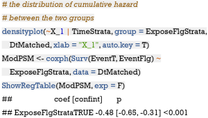
The result shows that the matched pairs have similar density distribution for X_1 (Figure 2) and the estimated coefficient (−0.48) is unbiased to the true effect size, and importantly the corresponding confidence interval includes the true effect. This method outperforms all previous methods in term of absolute bias.
Conditional logistic regression (CLR) model after sequential matching
Alternatively, the CLR model can be used to estimate the association between exposure and survival outcome after sequential matching (15). Recall that CLR is a specialized type of logistic regression usually employed when exposed/treated subjects with particular features are each matched with n control subjects with similar features. In our example, the exposed subjects were matched to control subjects with similar cumulative hazard within each TimeStrata. The matched dataset is stored in the data frame DtMatched.
The output shows that the estimated treatment effect is comparable to that estimated using Cox regression model after sequential matching.
Simulation study to compare PSs generated by treating treatment as binary and time-to-exposure variable
In the simulation study we compare two methods (i.e., those with and without considering the time-to-exposure property of the treatment) to calculate the PS, as the time-to-exposure property is always ignored in the literature, introducing the immortal time bias (16). After the comparison, we show the equivalence of time-dependent PS matching method and Cox regression model with time-varying covariates. The former is recommended as the first choice for such study design, because it also allows time-varying covariates to be included for the estimation of PS. Firstly, we define a function for the time-dependent PS matching.
The above chunk defines a function TDPSM() which receives a dataframe containing time-dependent exposure, covariates and survival outcome. The strataNo argument defines the number of strata for continuous recorded data. However, for follow up data at several fixed time points, the number of strata is not needed and we need to set StrataFlg = F to switch off the strataNo argument.The following chunk is to repeat the computation for a number of times (ii =100) to see whether time-dependent PS method is superior to the conventional PS method by treating treatment as a binary variable.
The above output shows that the coefficients obtained by survival model with time-varying covariate and by time-dependent PS matching are very close to the true value of -0.5. However, the coefficient obtained by treating exposure as binary variable is much greater than the true value, suggesting bias with this method. In the absence of time-varying covariates as in our example, both methods can be considered equivalently. However, time-dependent PS matching is recommended in the presence of time-varying covariates determining the hazard of exposure.
Application of time-dependent PS matching to the Kawasaki dataset
The Kawasaki dataset is a cohort of children with Kawasaki disease, which has been described elsewhere (17). A random sample of 500 cases is used for the illustration purpose. In the study we intend to explore whether time-varying standard treatment as represented by treat and treattime can help to ameliorate the coronary artery lesion (CAL). CAL is recorded as a time-to-event outcome with 1 stands for lesion presence and 0 otherwise. ytime represents the observation time. Other time-fixed covariates included:
- agemonth: age in month at presentation;
- gender: 0 for female and 1 for male;
- bithweight2: birth weight in kilogram;
- BMI: body mass index;
- feverday: duration of fever in days at presentation;
- keshi: whether there is transferring between departments;
- Kdgroup: 1 for complete and 0 for incomplete Kawasaki;
- preHB, prePLT, and preALB are laboratory findings for hemoglobin, platelet and albumin, respectively.
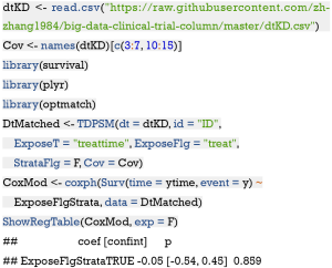
The result shows that there is no evidence to conclude that the outcome of patients between standard versus non-standard treatment is different. Readers can try to estimate the treatment effect with Cox regression model by treating the exposure as a time-varying covariate.
Conclusions
The article provides a comprehensive tutorial about the statistical tools to analyze survival data with time-varying exposures. We firstly simulate a dataset with time-varying exposure as a working example. Several approaches are performed to estimate the association between the exposure and survival outcome. Through simulation study, we found that the conventional PSM without considering the time-to-exposure property significantly biased the true effect because it did not take the time component into account. Multivariate adjustment with linear predictors from Cox and logistic regression model are also unable to estimate the true effect unbiasedly. Including time-varying exposure in a Cox regression model or creating matched cohort by time-dependent PS matching are recommended to reduce potential confounding bias. However, we still recommend the time-dependent PS matching approach because it also allows the inclusion of time-varying covariates affecting the hazard of exposure and also does not rely on strong model assumptions. After sequential matching with time-dependent PS, the treatment effect can be consistently identified by Cox regression model or CLR model.
Acknowledgments
Funding: This project is supported by the key soft science projects of Zhejiang Science and Technology Department (2019C25009).
Footnote
Provenance and Peer Review: This article was commissioned by the Guest Editor (Zhongheng Zhang) for the series “Big-data Clinical Trial” published in Annals of Translational Medicine. The article was sent for external peer review organized by the Guest Editor and the editorial office.
Conflicts of Interest: The series “Big-data Clinical Trial” was commissioned by the editorial office without any funding or sponsorship. The authors have no other conflicts of interest to declare.
Ethical Statement: The authors are accountable for all aspects of the work in ensuring that questions related to the accuracy or integrity of any part of the work are appropriately investigated and resolved.
Open Access Statement: This is an Open Access article distributed in accordance with the Creative Commons Attribution-NonCommercial-NoDerivs 4.0 International License (CC BY-NC-ND 4.0), which permits the non-commercial replication and distribution of the article with the strict proviso that no changes or edits are made and the original work is properly cited (including links to both the formal publication through the relevant DOI and the license). See: https://creativecommons.org/licenses/by-nc-nd/4.0/.
References
- Andersen LW, Granfeldt A, Callaway CW, et al. Association Between Tracheal Intubation During Adult In-Hospital Cardiac Arrest and Survival. JAMA 2017;317:494-506. [Crossref] [PubMed]
- Bender R, Augustin T, Blettner M. Generating survival times to simulate Cox proportional hazards models. Stat Med 2005;24:1713-23. [Crossref] [PubMed]
- Xu R, Luo Y, Glynn R, et al. Time-dependent propensity score for assessing the effect of vaccine exposure on pregnancy outcomes through pregnancy exposure cohort studies. Int J Environ Res Public Health 2014;11:3074-85. [Crossref] [PubMed]
- Austin PC. Generating survival times to simulate Cox proportional hazards models with time-varying covariates. Stat Med 2012;31:3946-58. [Crossref] [PubMed]
- Meira-Machado L, Faria S. A simulation study comparing modeling approaches in an illness-death multi-state model. Commun Stat Simul Comput 2014;43:929-46. [Crossref]
- Araújo A, Meira-Machado L, et al. GenSurv: Generating multi-state survival data 2015. Available online: http://CRAN.R-project.org/package=genSurv
- Terry M. Therneau, Patricia M. Grambsch. Modeling survival data: Extending the Cox model. New York: Springer, 2000.
- Zhang Z. Propensity score method: a non-parametric technique to reduce model dependence. Ann Transl Med 2017;5:7-7. [Crossref] [PubMed]
- Austin PC. An introduction to propensity score methods for reducing the effects of confounding in observational studies. Multivariate Behav Res 2011;46:399-424. [Crossref] [PubMed]
- Ho DE, Imai K, King G, et al. MatchIt: Nonparametric preprocessing for parametric causal inference. J Statistical Software 2011;42:1-28. [Crossref]
- Lu B. Propensity score matching with time-dependent covariates. Biometrics 2005;61:721-8. [Crossref] [PubMed]
- Hansen BB, Klopfer SO. Optimal full matching and related designs via network flows. J Computational Graphical Statistics 2006;15:609-27. [Crossref]
- Therneau TM. A package for survival analysis in 2015. Available online: .https://CRAN.R-project.org/package=survival
- Wickham H. Reshaping data with the reshape package. Journal of Statistical Software 2007;21. [Crossref]
- Andersen LW, Kurth T, Chase M, et al. Early administration of epinephrine (adrenaline) in patients with cardiac arrest with initial shockable rhythm in hospital: propensity score matched analysis. BMJ 2016;353:i1577. [Crossref] [PubMed]
- Lévesque LE, Hanley JA, Kezouh A, et al. Problem of immortal time bias in cohort studies: example using statins for preventing progression of diabetes. BMJ 2010;340:b5087. [Crossref] [PubMed]
- Shi H, Qiu H, Jin Z, et al. Coronary artery lesion risk and mediating mechanism in children with complete and incomplete Kawasaki disease. J Investig Med 2019;67:950-6. [Crossref] [PubMed]

