Propensity score matching with R: conventional methods and new features
What is propensity score analysis? Where is it used and why?
Where is it used?
It is essential to accurately estimate the effects of particular treatments or interventions in order to provide a solid evidential foundation for clinical practice. To this end, both randomized controlled trials (RCTs) and observational studies are commonly used tools.
RCTs can be characterized as scientific experiments that estimate treatment effects by randomly allocating subjects to two or more groups of differing clinical interventions, and comparing outcomes with respect to measured responses (2). Strategically designed randomized assignment reduces or even eliminates bias arising from the characteristics of subjects, clinicians, and administrators, or other confounding factors, and allows the effects of a particular treatment to be estimated by directly comparing outcomes between treated and untreated subjects. Therefore, randomization is the gold standard of causal inference (1-3). However, in some instances, RCTs cannot be implemented due to ethical issues, costs, and limited feasibility, which leaves the door open to implementing other new and innovative methods.
Observational studies have gained traction in recent years, owing to large amounts of available historical data, in which objects can be been observed, recorded, and compared, albeit without random treatment allocation (2,4). However, a major disadvantage of this approach is the presence of systematic differences in baseline covariates related to outcomes between treatment and control groups, which biases the results (1,5). To accurately estimate treatment effects from observational data, analysts have proposed several methods for balancing data, such as matching, stratification, and regression adjustments; however, each of these methods has its respective deficiency: (I) matching and stratification approaches group together individuals with the same or similar covariates, but these methods fail when too many covariates require balancing; i.e., it is difficult to find individuals for whom all covariates are similar. (II) For regression adjustments, it is often difficult to assess if models have correctly specified treatment assignments and covariates to outcomes. Goodness-of-fit measures, such as the coefficient of determination, R2 and mean squared error (MSE), do not test whether a model is correct for causal inference. Thus, a model that accurately predicts outcomes may still have biased estimates of treatment effects. Although regression is a simple and direct way to eliminate bias due to other factors, it is not entirely reliable.
What is propensity score analysis?
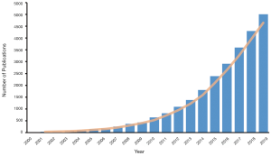
In recent decades, propensity score analysis (PSA) has attracted increasing attention (Figure 1). Propensity score (PS)1, as defined by Rosenbaum and Rubin, is the probability of receiving certain treatments, conditional on observed baseline covariates (6), and is estimated by using modeling to predict treatment allocation with covariates. In simple terms, PSA is based on the hypothesis that two patients with similar PSs have covariates which come from similar distributions. This means that by selecting or reweighting samples based on PS, researchers create new datasets where covariates are similar between treatment and control groups (7).
Methods including matching, weighting, stratification, and covariate adjustment based on PS all fall under the umbrella of PSA (8). For example, a complete analysis using propensity score matching (PSM) comprises six steps (Figure 2). The first step is to preprocess data sets, identify outliers, and interpolate missing values. In the second step, a model is specified, such as logistic regression, and trained on the dataset to predict whether a patient will be treated. For every patient, the trained model generates a probability of receiving treatment; i.e., his or her PS. The third step refers to matching based on PS, where different matching methods are tried, such as nearest neighbor, or optimal or genetic matching. In the fourth step, the balance of covariates between treatment and control groups is checked by calculating balance statistics and generating plots. A poor balance indicates that the model estimating PS needs to be respecified. In the fifth step, the treatment effects are estimated using matched data, and this is followed by the last step, where sensitivity analyses are performed to check the robustness of study results for hidden bias. These steps are later explained in detail.
What are the differences between PSA and other methods?
When compared with conventional balancing methods, PSA has two major advantages: dimension reduction and design separation. In PSA, dimension reduction means that multiple covariates are replaced by one score to describe a patient. In other words, when matching or reweighting patients, PS alone, rather than multiple covariates, is considered (1). Additionally, these methods separate covariate balancing and effect estimating. As shown in Figure 2, whether or not covariates are balanced between treated and untreated subjects should be checked in the fourth step, and treatment effects should be estimated after this.
Why should I read this tutorial?
While many PSA tutorials and PS articles have been published, there is room for improvement in this area. Some tutorials have provided step-by-step guidance, but cover just one or two packages (9-11), which limits their scope and practicality. Other articles and books have explained PS and related methods, as well as associated statistical principles and theories, but they explain little about the function usage in programming language, making the text difficult for readers to follow (1,8). In 2014 and 2015, Yao et al. (12) evaluated cancer studies (CS) and cancer surgical studies (CSS) using PSA, and found that many studies did not clearly provide the covariates required to estimate PS (CS 12.1%, CSS 8.8%), neglected comparisons of baseline characteristics (CS 21.9%, CSS 15.6%), or failed to report matching algorithms (CS 19.0%, CSS 36.1%). A systematic review by Malla et al. (13) observed that approximately 49% of articles through 2010–2017 (45% in 2016 and 2017) did not report imputation methods for missing data when applying PSM. Zakrison et al. (14) reviewed observational studies using PSA in the acute care surgery literature and found that more than 33% of studies did not adequately report their methods.
To this end, we composed this tutorial to introduce the PS concept and framework and to walk readers through how to implement PSM with R, with the aim of making readers capable of completing an analysis process using PSM.
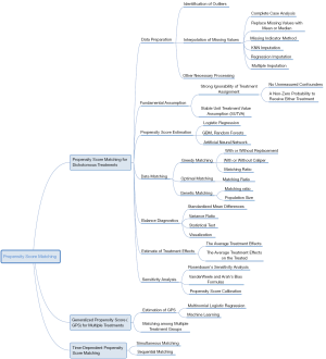
Our ultimate goal is to equip researchers with a comprehensive understanding of PSM, ranging from data preprocessing to PS estimations, from matching based on PS to the subsequent analysis, from generalized propensity score (GPS) for multiple or continuous treatments to time-varying PSM, etc. Unlike previous studies where technical details were either too brief or too abstruse, we have shown each algorithm in a simple manner, described the basic principles concisely, and illustrated steps using figures. Thus, this tutorial is a crucial document for clinical analysts. The mind map for causal inference with PSM is summarized in Figure 3.
Why choose PSM in R?
There are at least three reasons why this tutorial focuses on PSM: (I) several studies have shown that PSM eliminates a higher proportion of systematic differences in baseline characteristics between treated and control groups when compared with other methods (15-17); (II) PSM is more robust for the misspecification of the PS estimating model (3,18); and (III) PSM is the most commonly used PS method, having been implemented in many fields (12,14). It is worth noting that apart from the matching element of this tutorial, the PSM framework is similar to that of other PS methods; therefore, this tutorial is also valuable to readers wishing to try other PS methods.
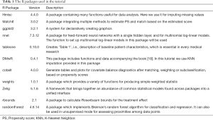
Nowadays, several programing languages including R (https://www.R-project.org/), Python (https://www.python.org/), and STATA (https://www.stata.com), support various PS methods. We have chosen R to illustrate how to perform PSM in different packages, as it is free, open-sourced, and user-friendly. We used the R version 3.6.2 for Windows (2019-12-12), which can be download from https://cran.r-project.org/. The package versions we used are listed in Table 1.
Full table
As some readers prefer to use other analytical tools such as Statistical Product and Service Solutions (SPSS) and Software for Statistics and Data Science (Stata), we provide package or tutorial recommendations for these tools in this part. We direct SPSS users to Huang et al. (19),who realized PSM in the PS matching module of SPSS and explain the analysis results. The software allows for the estimation of PS using logistic regression, and specifies options for nearest-neighbor matching, e.g., calipers, region of common support, matching with and without replacement, and matching one to many units. The program produces detailed statistics and graphs. For Stata users, psestimate, psmatch2, pscore, and other modules may be used for analysis. For example, psmatch2 implements full Mahalanobis and PSM, common support graphing, and covariate imbalance testing. Interested readers are directed to the package’s official documents.
The structure of this tutorial is as follows: Section ‘How do I start my PSM analysis when there are missing values in my dataset?’ covers data preparation, where we concentrate on methods for the interpolation of missing data for PSM. Section ‘How is PS estimated? What methods can be used?’ introduces approaches on how to estimate PS for dichotomous treatments using different models, such as logistic regression, random forests, and artificial neural networks. Section ‘How can patients with similar PSs be matched?’ concentrates on matching methods based on PS. Sections ‘What is a good match? Is my data balanced?’ and ‘What should be done if covariates are still unbalanced after matching?’ focus on balancing diagnostics after matching. Sections ‘How can the effects of treatment after matching be estimated?’ and ‘What about unmeasured covariates related to treatment allocation and outcomes?’ center on analysis after matching, including estimating treatment effects and sensitivity analyses. In Section ‘How does PSM handle multiple or continuous treatments?’ and ‘How to apply PSM with time-dependent covariates and treatments’, we introduce GPS for multiple or continuous treatments, and time-dependent PSM. In the last section, we discuss PSM in terms of strengths and weaknesses, and we assess the limitations of this tutorial.
How do I get access to data from this tutorial?
To illustrate PSM in R, we constructed a dataset with known true PS values, for step-by-step guidance in each section. This dataset simulates the relationship between smoking and cardiovascular disease (CVD), with age and gender as the potentially confounding covariates. However, one must bear in mind that real data is not as simple as the simulated data in this tutorial, in which only two confounding factors are present. We will cover how to determine covariates from hundreds of variables in observational datasets for estimating PS (Section ‘Selection of covariates’).
In a hypothetical situation, we want to study the relationship between smoking and CVD incidence. Thus, CVD is the outcome variable (CVD = 0 when the patient does not have CVD; otherwise, CVD =1). Smoking is a binary variable which indicates whether the patient smokes or not. Gender (0= female, 1= male) and age are two confounding covariates, which are correlated to “treatment”2 and outcome. Now, we assume that men smoke more than women, and middle-aged people smoke more than elderly and younger people. Lastly, we randomly set variable values as NA (missing).
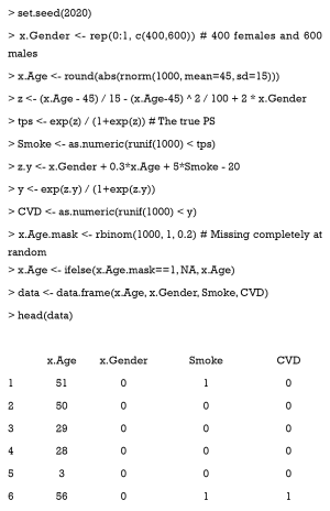
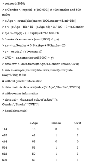
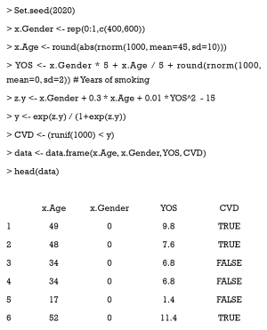
Data is generated with the following code:
Here, tps is the true PS which can balance data and needs to be estimated.
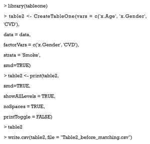
Next, we use the CreateTableOne function in the tableone package, to summarize the distribution of baseline variates in each group, and test whether significant differences exist between different groups. If you do not have tableone, it can be installed with the following code: install.packages (“tableone”). The results of following code are shown in Table 2.

Full table
Here, the argument vars is a vector of variables to be described, factorVars is a vector of variables that should be handled as categorical variables, and strata is the column name that groups the data set. As can be seen, the covariates of age and gender are significantly different between the smoking and non-smoking groups. The SMD column refers to standardized mean differences between different groups, which is calculated by the following equations.
For continuous variable x:
where and are the sample means for the treated and controlled groups, respectively; Var1 and Var2 are sample variances for the treated and controlled groups, respectively.
For dichotomous variable x:
where and are the prevalence of dichotomous variables in the treated and control groups, respectively.
The use of SMD is recommended to measure the covariate differences between different groups when using PSM. It provides a fair scale to compare different types of covariates that are not influenced by the units of measure, because it standardizes the differences based on the variance of the samples.
How do I start my PSM analysis when there are missing values in my dataset?
Data preparation is the first step in PSM, as outliers or missing values will impede an accurate PS estimate. Although some models, like XGBoost, are immune to missing values, they are rarely used in estimating PS; meanwhile, common models, such as logistic regression and artificial neural network, cannot deal with missing values. Therefore, in this section, we focus on missing data, and demonstrate and compare different methods for missing values.
How do I deal with missing values?
In theory, missing data may be classified as missing completely at random (MCAR), missing at random (MAR), and missing not at random (MNAR) (20), but these classifications are not focused on here. Complete case analysis is a simple method to deal with missing data. It deletes cases with missing values, and is based on the assumption that data are MCAR, and they substantially reduce sample size and increase variance (20,21). The approach is not recommended, particularly for small-data analyses, or when miss ratios are high. The missing indicator method replaces missing values with a constant, usually 0, and adds missing indicators for each imputed covariate. This method has been criticized as it usually introduces bias (22). Replacing missing values with the mean, median, or mode is also widely used. Despite its simplicity, the approach reduces variability in the data set, and underestimates variance (8,21). The K-nearest neighbors (KNN) and random forests are machine-learning methods that can be used to impute missing values (23-25). In addition to these, model-based single imputation methods, such as regression imputation, or matching-based single imputation methods, such as hot-deck imputation, are better-designed, but they amplify correlations in the data (8). Several studies (8,20,26) recommend multiple imputation (MI) to impute missing data, because this method does not reduce inherent variability.
Although MI is currently the preferred missing data imputation method, there is still debate as to which method is the most appropriate for PSM (8,27,28). In a simulation study, Choi et al. (29) compared four different methods: complete case analysis, the missing indicator method, MI, and combining MI and the missing indicator method. These authors found that MI would fail when data were non-randomly missing, and the optimal way to handle missing values depended on the missing data structure.
Combining MI and PSM is another contested issue. First, it has been recommended (30) to separately impute data for treatment and control groups, as missing mechanisms and covariate distributions may be different between these groups. However, this approach was not mentioned in recent studies (29). Its major disadvantage is that separate imputation mechanism reduces the sample size for imputation to each group, which biases the imputed values. Meanwhile, two methods that implement PSM with multiple imputed data have been compared (7). In the first, PSM is separately applied to each dataset imputed by MI, and the treatment effect estimates are averaged. In the second, PSs on each completed dataset are estimated, the scores for each record are averaged, and PSM is performed with averaged scores to estimate treatment effects. This second method has the greater potential to produce substantial bias reductions.
How do I implement missing data methods with R?
Checking missing values
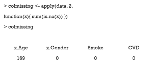
Here is a simple way to count the number of missing values in each column.
As can be seen, there are 169 missing values in the column x.Age.
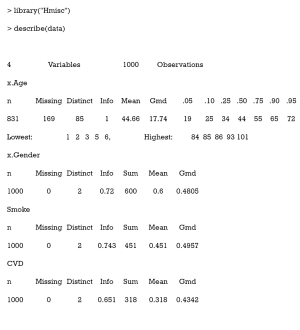
The Hmisc package contains several functions for data analysis. The data may be summarized as follows:
Gmd refers to Gini’s mean difference, which is a robust measure of dispersion. The reader is directed to (31) for more information.
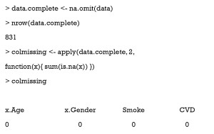
Completing the case analysis
The function na.omit returns a new data frame which contains samples without missing values.
As can be seen, those samples with missing values are deleted.
Replacing missing values with mean, median, or specified constant
The use of the impute function in the Hmisc package is straightforward.
The missing indicator method
The missing indicator method is a simple approach,
where x.Age.ind indicates Age (1 = missing, otherwise 0)
The KNN imputation
For every patient with missing values, this algorithm finds the top k similar patients as the nearest neighbors, and then uses the covariate values of neighbors to impute the missing ones. Now, we use the knnImputation function in the DMwR package to implement KNN imputation. The argument k is the number of neighbors, and the option meth = “weighAvg” means that the nearer neighbor will be given a larger weight to impute.
Multiple imputation
The MI approach is more complex than the above-mentioned methods. The code is hard to understand unless the user knows how to match patients based on PS. Therefore, we have provided the PSM code with MI attached in the appendix for reference.
How is PS estimated? What methods can be used?
The PS is the conditional probability of receiving a treatment, given a vector of observed covariates, X. In this section, we discuss the simplest case, where two treatment options (binary) are provided; i.e., treatment vs. control.
A common method to estimate PS is to build a model and predict treatment assignment based on covariates. First, appropriate covariates are selected, and a modeling method, e.g., logistic regression, is specified. Then, a predictive model is trained on the data using the selected covariates to predict whether a patient will be treated. Lastly, the model makes predictions for each patient, and PS is the probability of receiving treatment, as predicted by the model.
In the following paragraphs, we demonstrate covariate selection, the methods to estimate PS, and how to estimate PS with R.
Selection of covariates
Not all covariates need to be balanced. According to the theory of casual inference (32,33), we can analyze the different relationships between the covariate (X), the treatment assignment (W), and the outcome (Y). As demonstrated in Figure 4, the X covariates in the first row (I, II) should be included in the estimating model, while those in the second row (III, IV) should not.
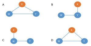
- This X is the true confounding variable in the data. If we suppose that older patients are more likely to be given intraoperative blood transfusions (W) but with a higher mortality risk (Y), we observe then that blood transfusions caused significantly more deaths in the historical data. Age is a true confounder, and should be balanced between the transfusion and non-transfusion groups; otherwise, the results will be biased.
- Although there is no direct causal relationship between X and W, several simulation studies suggest that these covariates should always be included in a PS model. The inclusion of these variables will decrease the variance of the outcome estimates, without increasing bias (34,35).
- In contrast, including variables related to the treatment but not to the outcome, will increase the variance of the estimated exposure effect, without decreasing bias (34).
- This X is a mediating variable in the causal path from W to Y; i.e., W affects Y by X. For example, if we want to study the effects of cigarettes on the risk of lung tumors, X refers to the nicotine intake of each individual per day, Y is the average number of cigarettes smoked per day, and Y is the lung tumor indicator. Nicotine is a powerful poison in cigarettes. People who inhale high levels of nicotine can damage their lungs (W->X->Y). If X is balanced between the smoking and non-smoking groups, then the effect of W on Y will be underestimated or even eliminated.
Unfortunately, domain knowledge must be applied to ensure all important confounders are included in an analysis, as doing so solely by automatic computer script is impossible (36).
Estimating methods
Binary logistic regression is the mainstream PS estimating method, but an increasing number of alternative methods are being proposed, including bagging or boosting (31,37), recursive partitioning algorithms (31), the generalized boosting model (GBM) (37,38), random forests (31), and artificial neural network (ANN) (39).
The most significant advantage of logistic regression (LR) is its simplicity and interpretability. To illustrate, in an observational study, older patients are more likely to be assigned to a treatment group, and younger patients to control groups. Thus, for outcomes, mortality is correlated to age. Accordingly, you can model the treatment assignment as a function of age using LR, and estimate PS with your prediction model.
Now let us assume the situation is more complicated: older patients and children are more likely to be treated than middle-age patients. If researchers use LR without careful thinking, estimating PS could be biased because the relationship between treatment assignment and age is no longer linear. In this case, an experienced researcher will add polynomial or interaction terms to the model to fit more complicated relationships between covariates and treatment assignments.
Therefore, after we estimate PS and match based on it, a data balance diagnostic is required to guarantee that the model is well specified to eliminate confounding factors. This step is introduced in section ‘How can patients with similar PSs be matched?’.
The estimation of PS by LR is time-consuming, because different polynomial or interaction terms must be determined to balance the data. While no method is optimal, machine learning may help. GBM, random forests, and ANN automatically fit complex and high-order relationships in data, which frees researchers from having to find the best model structure (39-42). For example, ANN is composed of one or more layers, in which data are transformed in linear and nonlinear ways, and so ANN is more flexible for data mining than LR. In the literature, Westreich et al. (42) and De Vries et al. (43) observed that the use of classification and regression trees (CART) is promising for PSA application. Simulation experiments by Keller et al. (41) indicated that ANN performed similarly to LR when the LR model was correctly specified, but when the LR was inadequately specified, it was outperformed by ANN. Recently, Super Learner, an ensemble machine learning algorithm, was shown to be robust for the misspecification of the PS estimating model (44).
Although machine learning methods are criticized because of their poor interpretability, we argue that more attention should be paid to whether the estimated PS balances the observational data, rather than what the relationship is between the covariates and treatment assignment. Therefore, these “black box” methods may be promising alternatives to LR. Nonetheless, there is much to explore and research concerning PSM and machine learning methods (8).
Estimating PS with R
MatchIt package
The MatchIt package offers users practical functions to estimate PS. We recommend first installing the package and uploading it.
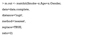
matchit is the main function in MatchIt, which can estimate PS and match similar patients. It is used as follows:
The argument formula follows the usual syntax of R formula, which specifies the PS estimate model in which treat ~ x1 + x2, where treat is a binary treatment indicator, and x1 and x2 are pretreatment covariates; i.e., Smoke ~ x.Age + x.Gender.
Distance is the key argument that decides what model you will use to estimate PS, and can include “logit” (logistic regression), “GAMlogit” (generalized additive models), “rpart” (CART), and “nnet” (single-hidden-layer neural network model). Also, Distance may be PS estimated by the researcher. This means that PS can be estimated with other models in other packages, and the function, matchit, can be used to match patients based on your estimated PS. It is worth noting the option “mahalanobis” (Mahalanobis metric distance), which is not a method based on PS. In fact, Mahalanobis metric distances were developed and studied prior to PSM (45,46). They play a similar role as PS in assessing the similarities of different patients.
An optional argument, distance.options, specifies parameters for estimating models. The input of this argument must be a list. Table 3 lists those parameters that can be set. Some are optional, while others must be set if you want to use this model. The matchit function completes both PSM estimations and matching steps. However, here we refer to the estimation only. How to match and set other arguments such as method and discard will be covered in the next section.

Full table
Running matchit with logistic regression
We then use the following code to run matchit. As mentioned previously, we do not set other arguments, except distance. We use complete cases in our dataset for the following steps, because x.age is missing completely at random and our data of just two columns is so simple that it leads to the poor performance of other imputation methods.
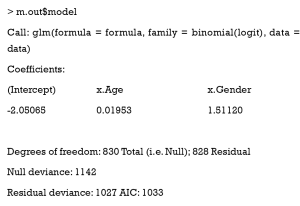
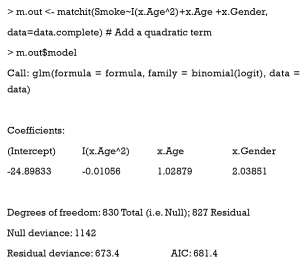
The value model of m.out can be checked to get the summary of the estimating model. This is the summary of our logistic regression.
The value distance will return the estimated PS for each sample, which is a vector of length n (PS is considered as the distance of patients to match here).
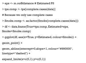
Now, we compare the estimated PSs with the true values.
In the scatter plot in Figure 5A, the x-axis is the true PS value, while the y-axis is the estimated value. The small circles represent samples. If PSs were estimated accurately, these circles would be distributed around the line y = x. The reason why the estimation is so poor (like a sin function), is because we generated PS by quadratic equation, but estimated it by linear equation. We can change our model to fit the nonlinear relationship, so it can be operated by the following code. Note that when we use PSM with real datasets, we do not know how the true PS is distributed, so this adjusting of the model by logistic regression may take more time.
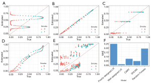
As seen in Figure 5B, when the correct model is specified, PS is accurately estimated.
Running matchit with CART and a neural network
Now, we will show you the estimating results of CART and a single-hidden-layer neural network (Figure 5C,D, respectively). Only the call of the matchit function is shown here, as the remaining codes are all the same.
Then, we change the distance argument to “nnet”, and set the number of hidden-layer units as 16.
Although the true PS is generated in a complex manner, the CART and neural network can also estimate the score based on x.Age and x.Gender. In practice, when we do not know how the true PS was generated, logistic regression is not always perfect, while neural networks can estimate better scores based on baseline covariates.
Estimating PS by other functions
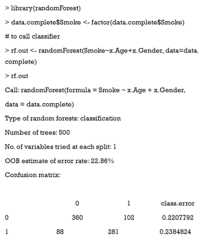
Apart from calling the built-in function of MatchIt, PS can also be estimated using the model you specify, like any other dichotomous problem. In this section, we use random forests, a popular ensemble algorithm based on decision trees. Several R packages support random forests; here, we chose the package randomForest.
We use the fraction of votes as treatment probabilities, namely, PSs.
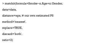
As shown in Figure 5E, the random forests performances are unsatisfactory. After we calculate PS with our model, the matchit function may still be used to match data, based on the estimated PS:
Different models in terms of estimating accuracy are summarized in Figure 5F, but one example cannot show their performances in all situations.
How can patients with similar PSs be matched?
Matching methods
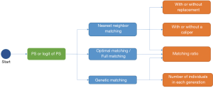
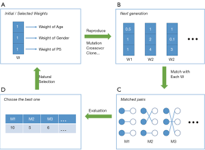
After we calculate PS, we form pairs between treated and untreated subjects, according to their PSs. There are several ways to do this, but several choices must first be considered, as outlined below. We have summarized an idea map for choosing matching methods (Figure 6), and compared matching results of different algorithms (Figure 7).A separate flowchart (Figure 8) illustrates how genetic matching works because it is more complex.
PS or logit of PS
Early in 1985, Rosenbaum and Rubin (47) suggested using the logit of PS (i.e. ,) to match samples, because the distribution of logit PS approximates to normal, although matching based on PS is still feasible.
Major matching algorithms
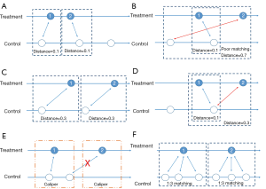
Nearest neighbor matching (NNM) is a widely used method, and is composed of two steps. First, the algorithm picks patients, one by one from treatment groups, in a specified order. Then, for each treated patient, the program finds a patient in the control group with the nearest PS. These steps are repeated until no patients are left in the treatment or control group. As shown in Figure 7A, “1” is selected first, and matched to an untreated subject. The distance between their PSs is the smallest (0.1). Then “2” is selected and matched.
The essence of this method is that it divides the whole, complex, matching problem into small parts, matching one treated subject at one time, and determining the best counterpart every time. The method is considered “greedy” because it is greedy in every subproblem (i.e., it finds the best one), yet overall optimal output is not guaranteed. As shown in Figure 7B, the algorithm picks “1” first and “2” next. For “1”, the algorithm finds the best untreated patient to match, their PS difference is 0.1. However, for “2”, the distance is much worse. An observer may conclude that if we deal with “2” first and then “1”, an optimal matching situation will result (Figure 7C). Indeed, different orders for patient selection have been proposed, such as from the highest to lowest PS, from the lowest to highest PS, or random order. However, simulation experiments have demonstrated that the order in which treated subjects are selected for matching exerts only modest effects on estimations (48). Equally, other methods have been proposed to alleviate this problem, such as specifying a caliper width (discussed later). Despite suboptimal performances, NNM is used extensively by researchers for PSM. It is a simple algorithm to understand and implement, and when there are sufficient untreated patient numbers, these poor matching issues are unlikely to happen.
In contrast to NNM, optimal matching (OM) was proposed by Rosenbaum (49) to optimize total distances between treatment and control groups. This means that algorithms determine matched samples with the smallest average within-pair absolute difference in PS (Figure 7C). Determining optimal matches is implemented using network flow theory (50,51), but this is beyond the scope of this tutorial. Gu and Rosenbaum (52) observed that OM was sometimes better than NNM as it produced closely matched pairs, but was no better than NNM in terms of balancing covariates. In a comparison of 12 matching algorithms (48), OM induced the same balance in baseline covariates as NNM, suggesting both NNM and OM are potential candidates for matching.
Strictly speaking, genetic matching (GM) is the extension of PSM (Figure 8). The algorithm considers not only PS, but also specifies covariates and determines a set of weights (i.e., variable importance) for PS and each covariate (53). In our data, for each patient, we recorded age, gender, and estimated the PS. If the weight of age was set to 2.5, while the weights of gender and PS were both 0.5, then the differences of age within the matched pairs will be paid 5 times more attention to than those of gender and PS. The PSM may be considered a limiting case of this method, in the sense that when all the weights of other covariates excepting PS are set to 0, GM will be equivalent to PSM.
It is obvious that weights must be meticulously designed to balance covariates. The GM uses an evolutionary search algorithm to determine sets of weights for each covariate, and achieves data balancing based on weighted covariates (53), which is why it is called “genetic”. As shown in Figure 8, GM starts from the initial sets of weights (the parents’ genes). Second, GM randomly modifies some weights in these sets (mutation), and randomly recombines them with each other (genetic recombination) to generate the next generation of weights. Third, samples are matched with each set of weights to generate the same number of matching plans as individuals in the generation. Then, one solution which optimizes the data balance can be selected (natural selection). These steps are repeated until covariate balancing is achieved, or the maximum number of iterations is reached. Every candidate generation evolves, and the algorithm asymptotically converges towards an optimal solution.
In addition, several methods have an ambiguous relationship with PSM. For example, exact matching (EM) is a method that matches treated with controlled patients, using the same values of specified covariates. The method is used when only a few covariates may influence the treatment assignment. When the number of covariates increases, even though covariates are all binary, the number of possible matches grows exponentially, resulting in a poor matching result. Technically, EM is not a kind of PSM, but in Section ‘What should be done if covariates are still unbalanced after matching?’, we will explain how to use PSM and EM together.
Note that subclassification and full matching (FM) are often classified as matching methods (9,10). In fact, these methods are also regarded as stratifications based on PS, and are another series of methods that reduce selection bias in observational studies (1,3). Subclassification methods stratify patients into several groups, based on their estimated PS. Patients in one group will have similar PSs, and therefore differences in covariates can be ignored.
FM is a subclassification approach that optimally forms subclasses, which is the reason why it is also called optimal full matching (51,54,55). Each subclass contains 1 treated subject and 1 or more control subjects, or 1 control subject and 1 or more treated subjects. The subclass may be viewed as a matched set where 1 subject is matched to 1 or more counterparts, and thus can be construed as a matching method.
NNM with or without replacement
Matching with replacement means that after a patient from the treatment group is matched to another from the control group, the controlled patient is reintroduced to the control group for next-round matching; therefore, a patient in the control group may be used more than once (Figure 7D; red arrow). In contrast, matching without replacement means that after matching, the matched pair from the candidate pool will be removed such that a participant in the control group will be used only once.
NNM with or without a caliper
Matching with or without a caliper determines whether the upper limit of the distance of PSs in a matched pair will be set or not. When the PS distributions are considerably different between the treatment and control groups, the distance of PSs in a matched pair may be large, as is the case in Figure 7B. Then, a caliper must be added into the matching step. Thus, for every patient, they can only be matched to patients of a PS within a limited range (Figure 7E). If eligible patients cannot be matched, the patient should be discarded.
While there is no gold-standard for maximal acceptable differences, a simulation study by Austin suggested that a caliper width of 0.2 of the standard deviation (SD) of the logit of PS be used, as this minimized the MSE of the estimated treatment effect, in a variety of settings (56). We suggest that (I) if the matching performance is poor (e.g., a few covariates are not balanced) matching can be conducted with a tighter caliper and (II) if matching is successful but the number of matched pairs is small, the caliper width can be broadened.
Pair matching, or other matching ratios
In pair matching, each treated patient matches to a single control in 1:1 ratio. Moreover, the ratio of controls to treated patients can be n:m (n and m are integers). For matching using variable ratios, each treated patient matches to, for example, at least one and at most four single controls (e.g., full matching). Figure 7F shows a 1:3 matching.
Matching with R
The function matchit of the MatchIt package implements both the estimation and matching steps of PSM. In Section ‘How do I start my PSM analysis when there are missing values in my dataset?’, we introduced PS estimations; here, we discuss matching.
Arguments
The use of matchit is as follows:
The argument method specifies the method used to match patients, passing string values including “nearest” (nearest neighbor matching, the default option), “optimal” (optimal matching), “genetic” (genetic matching), “exact” (exact matching), “subclass” (subclassification), and “full” (full matching).
The reestimate is a logical argument. If TRUE, after we discard unmatched samples, and PS is re-estimated with the remaining samples. This will not occur if this argument is FALSE or missing. In addition, we tabulate additional arguments for each matching method (Table 4).

Full table
Examples
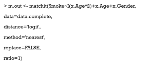
Next, we perform a simple match to see the outcome of matchit. It is worth noting that if you use optimal matching, the optmatch package must be installed, while genetic matching requires the rgenound package.
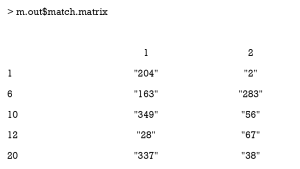
This is an example of NNM. Matched pairs can be checked as follows.
Each row represents matched pairs of a patient in the treatment group. In each row, the first number indicates the serial number of the treated patient; numbers on the right are the controlled patients matched to this patient.
The value discarded records whether this patient was discarded.
What is a good match? Is my data balanced?
Balance diagnostics
After PS-based matching, a new dataset is generated; however, there is no guarantee of data balance. In this section, we investigate how to check balance in covariate distributions between treatment and control groups. Herein, we introduce and compare various balance diagnostic methods, followed by practice using R software. Note that we have not modified our PS model, and therefore some covariates remain unbalanced. In the next section, we discuss practical methods to cope with poor balance.
A direct and preferable method is to compare standardized mean differences (SMD) and variance ratios (VR) of covariates in the treatment and control groups (11). In the preceding context, we introduced SMD, which is an important metric that measures covariate differences between different groups, because it is not influenced by units of measure. Stuart (27) recommended that a covariate is balanced only when the absolute SMD value is <0.25, while Austin (3) proposed a more stricter criterion that it should be <0.1. The VR is the ratio of variance in the treatment and control groups. A VR close to 1.0 indicates a balance in the covariate, whereas a VR <0.5 or >2.0 are considered “too extreme” (57).
Significance testing is another widely used method, and the test results after matching are shown in many studies with PSM (58-60). However, it has been criticized that the increase of P value may be due to the decreasing sample size of the study population after PSM (11,61-63). Several studies have argued that we should use statistics that account for a matched design, such as a paired t-test for continuous outcomes and McNemar’s test for dichotomous outcomes in 1:1 matching design (14,64). This practice is rarely implemented or explicitly stated in the literature. Herein, rather than settling this dispute, we provide ways for researchers to conduct more in-depth research.
Graphical methods such as histograms, quantile–quantile plots, cumulative distribution functions, and love plots have also been proposed to show and check covariate distributions in a visual way.
It is worth nothing that goodness-of-fit measures, such as c-statistics, or area under the receiver operating characteristic curve (AUROC), indicate only the degree to which PS models discriminate between treated and untreated patients. However, these statistics provide no information as to whether PS models are correctly specified (3).
Balance diagnostics with R
SMD and VR
The summary command
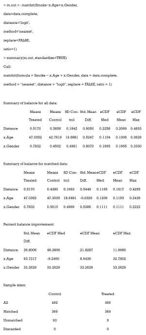
The easiest way to calculate SMD and check covariate balance is to use the summary command on the output of matchit. This command provides an overall measure of the balance between treatment and control groups in the original and matched data set. Three options in the summary command may be used to check balance and respecify the PS model: (I) With the option interactions = TRUE, the output summarizes the balance of all squares and interactions of covariates in the matching procedure. Large differences between the treatment and original groups usually indicate that these items should be added into the PS model in order to achieve data balance. (II) The option addlvariables = TRUE shows the balance of covariates not used in the PS model. Similarly, these covariates should be included in the model if large differences are observed. (III) The option standardize = TRUE prints out standardized versions of the balance measures; i.e., the SMD where the mean difference is divided by the SD in the originally treated group. We suggest that standardize = TRUE should be set to compare the covariate balance in a scale-free way.
The output from the summary command includes five parts: (I) the original assignment model call; (II) a data frame which shows the mean of the distance (PS) and covariates in the original treatment and control group, the SD in the control group, the (standardized) mean difference between the two groups, and the median, mean, and maximum differences in cumulative distribution functions (CDFs) for each covariate; (III) a data frame which contains the same statistical items as above, but for the matched data set; (IV) percent balance improvement before and after matching; and (V) a data frame which counts samples, in all (original) data sets, which are matched, unmatched, or discarded.
As observed, after matching, age is balanced (0.0329<0.1) while gender is not (0.5386>0.1). Although discrete variables are allowed in the Matchit function to estimate PS, they are considered as continuous to examine balance in the summary (e.g., to calculate SMD). That means that the summary command indiscriminately calculates the SMDs of discrete and continuous variables, leading to bias for discrete ones.
CreateTableOne
When generating simulation data, we used the CreateTableOne function to calculate SMD. However, we do not recommend using it for matched data, because this function only takes matched data into account, and the mean difference is standardized (divided) by the SD in the matched data. After matching, it is probable that the standard deviation will be smaller in the matched data, so that the SMD may be larger than before matching, although the mean difference decreases (11). This means SMD is overestimated by CreateTableOne. A better way is to use the original SD, which is implemented by the bal.tab function in cobalt package. This will be introduced later.
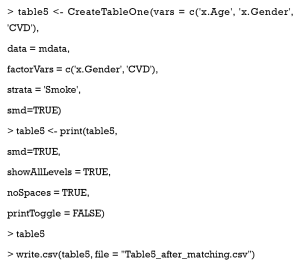
Nonetheless, we created Table 5 to summarize baseline covariates of matched data, using the CreateTableOne function. Firstly, we exported our matched data from Matchit.

Full table
We then created a summary table.
Here, the SMD of gender is 0.487, which indicates this covariate has not been balanced.
The cobalt package
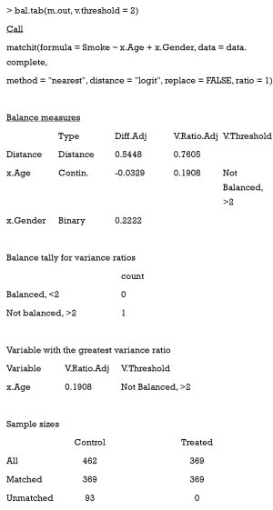
The function bal.tab in cobalt package provides a useful way to calculate SMD. After the package is installed, the following code can be used.
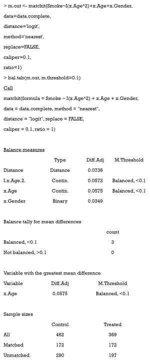
Here, the argument m.threshold is a numeric value for the SMD threshold. This function shows which covariates are balanced (SMDs are under the threshold), which covariates are unbalanced, which covariate has the greatest mean difference, and the sample size of the matched data. The SMD of age is the same as that calculated by summary (m.out), while the SMD of gender is calculated as appropriate for binary variables. When comparing SMDs of gender from Table 5 with those here, we observed that the former SMD (0.487) was twice as much as the latter (0.2222). As previously mentioned, the mean difference was standardized by the SD in the different datasets, and thus the result from the function bal.tab was more credible.
The VR can be calculated and checked by setting the argument v.threshold, which is a numeric value for the VR threshold. As previously mentioned, a good VR is 0.5–2. In this function however, if VR is < 1, it will be converted to the inverse (1/VR). Therefore, we just need to set v.threshold = 2.
The VR is not calculated for the binary covariate gender, and age is not balanced according to the VR criterion.
Statistical significance
CreateTableOne
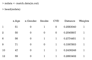
Now, we need to export out matched data, using the match.data command.
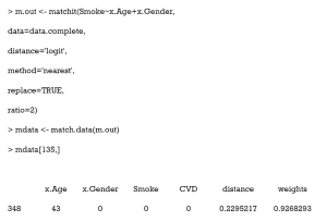
Here, the first 6 columns are the original columns from our data frame. The Distance column is the estimated PS, while the Weights columns is the weight each sample was given. These weights were calculated by well-designed rules, to ensure that the matched treated and control groups were similarly weighted. Because we chose 1:1 matching without replacement, all weights were assigned as 1. Otherwise, these weights were calculated according to how many times a unit was used to match. There will be problems if matching ratios are not 1:1, or we match with replacements. An example of this is as follows:
As can be seen, 1 participant (no. 348) was matched several times and had a weight of 0.927 in the exported data. Statistical tests with weights can be performed to check balance in this case by using weighted t-tests with the wtd.t.test function in the weights package, for instance.
Paired t-tests
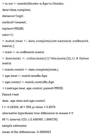
If paired t-tests are to be used, the order of covariate values should be sorted, and the t.test function used with paired = TRUE. Here we provide a simple example:
Kolmogorov-Smirnov (KS) statistics
The function bal.tab in the cobalt package also provides KS tests, which compare the distribution of covariates between treatment and control groups. The only requirement is to set the ks.threshold parameter.
Distribution visualization
The plot command
The plot command has three different options; the Q–Q plot (default), the jitter plot (set type = ‘jitter’), and the histogram (set type = ‘hist’). The Q–Q plots demonstrate deviations between empirical distributions of treated and control groups. The points in Q–Q plots lie on the y = x line. Larger deviations indicate greater differences between the distributions. Jitter plots show the PS distributions of unmatched treatment units, matched treatment units, matched control units, and unmatched control units. Every circle in the jitter plot represents a patient, and its size is proportional to its weight given by the matchit function. The distributional density of PS before and after matching is shown in histograms. The results are not shown in this tutorial.
The cobalt package
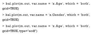
Variable distributions are visualized using the bar.plot function.
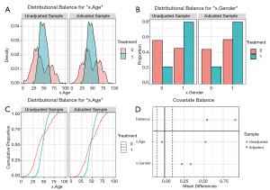
The density plot is displayed for continuous variables (Figure 9A), while for categorical variables, a distribution histogram is displayed (Figure 9B). Empirical cumulative density function plots are drawn by selecting type =“ecdf” (Figure 9C).
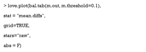
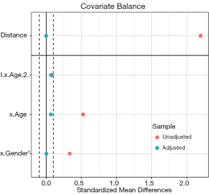
Love plots compare SMDs of covariates before and after matching, where two vertical dotted lines are drawn as the 0.1 threshold of SMD, and every point represents the SMD of a covariate before or after PSM adjustment. If a point lies between two lines, then the corresponding covariate has been balanced. Herein, we used the love.plot command of the cobalt package to draw Figure 9D. This subfigure represents the visualization of SMD results calculated by the bal.tab function in Section ‘SMD and VR’, where the SMDs of age and gender are –0.0329, and 0.2222, respectively.
As shown in Figure 9D, the variable x.Age is balanced, while x.Gender is not. It is common to encounter unbalanced covariates when using PSM. In Section ‘What should be done if covariates are still unbalanced after matching?’, we provide several practical methods to deal with unsuccessful matching.
What should be done if covariates are still unbalanced after matching?
There are at least five methods to help PSM balance data.
- The first method is the most commonly used. It respecifies the model to estimate PS; e.g., it adds high-order or interaction terms, or changes to another modeling method. For example, in the preceding code, we used Smoke~x.Age+x.Gender to estimate PS, but it was not precise. Then, we added a quadratic term to our model, but unfortunately, the result was still poor.
- The second method is to change the matching method. For example, it is worth trying NNM with a tighter caliper, but this may shrink sample size.
- (III) The third method combines PSM with an exact matching method, by setting exact=c('x.Gender') in matchit. That is to say, when matching patients with similar PSs, some covariates (gender) must be equal. The effect of this method is not ideal; therefore, we do not use it.
- The fourth method is to increase sample size, usually by collecting more data. In a scenario where there is 1 male and 1 female, regardless of the method used, they cannot be matched with a balanced gender. Therefore, with more data, matching should become easier.
- Lastly, residual differences in baseline covariates after PSM can be handled by conventional methods such as matching, stratification, regression adjustment, and so on (3,8,38). In other words, we balance our data successively by PSM and conventional methods (59).
In real data, with many more variables, it may be difficult to find the correct formula to estimate PS. Researchers have to try different covariate combinations. The command summary (m.out, interactions = TRUE, addlvariables = TRUE, standardize = TRUE) provides balanced interaction information and high-order terms of all covariates, but as covariate numbers increase, the result table will be harder to comprehend. Also, a few methods serve as indicators for high-order relationships, such as car and gvlma package in R. In addition, most machine learning methods can automatically learn rules of data and fit complex relationships between variables, which is their major advantage.
As can be seen, covariates are all balanced, but we lost almost half of the treated samples [197].
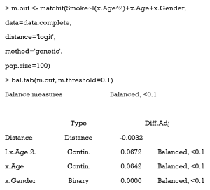
After adjustment, we can observe that using GM with pop.size =100 balanced our data with all treated samples matched.
A love plot of SMD is shown in Figure 10. As can be seen, the PSM performance was much improved when compared with the one before. There are three reasons for this: (i) the former model to estimate PS was incorrect (the model was linear, while the correct one was quadratic). Herein, we used the correct model to estimate PS. (ii) The matching algorithm of the latter was GM, which outperformed the ordinary matching algorithm in this case. (iii) Here, each treated patient was matched to fewer than 10 controlled individuals, while in Figure 9, only 1:1 matching was implemented.
How can the effects of treatment after matching be estimated?
What is the meaning of treatment effects in non-randomized experiments?
Under the counterfactual framework proposed by Rubin (65), for every individual, there are two kinds of potential outcomes (under treatment or control conditions) before treatment assignment. Once the patient receives a treatment or control, researchers observe one of two outcomes, but the other is missing. To some extent, data analysis in observational studies is like the interpolation of missing outcomes.
Abadie and Imbens proposed an estimator of treatment effects appropriate for matching (66,67). In the matched data, all covariates have similar distributions between treatment and control groups. That means the matched patients are considered similar. Missing outcomes of the treatment group are interpolated using the mean outcomes of the matched controlled group, and vice versa. Suppose patients who received treatment have a mean outcome (A). After PSs are estimated and matching is performed, we interpolate outcomes of the treated patients under control conditions with matched patients’ outcomes. If they had not received treatment, the expectation of their outcome should have been B. Thus, we compare the two mean outcomes (A vs. B) on matched data to estimate the average treatment effects on the treated.
How can treatment effects be estimated with PSM?
Generally speaking, two kinds of treatment effects are of concern: the average treatment effect (ATE) and the average treatment effect on the treated (ATT). Whether ATT or ATE is estimated depends on which is of interest and what matching method is used. Some believe that PSM only estimates ATT (27,68,69). For instance, if NNM is used, for each treated patient, the most suitable untreated patients are matched. By averaging the outcomes of the controlled which are matched, the missing potential outcomes for treated patients is actually estimated, and therefore ATT is estimated. However, in the official document of the MatchIt package (70), authors have provided an example where they estimated ATE using NNM and the Zelig package, which estimates causal effects by Monte Carlo simulation. A detailed explanation of this is beyond the scope of this tutorial. Also, if subclassification or FM with matchit function is used, patients are grouped into several subclasses based on their PSs, and thus ATE can be estimated.
When estimating effects, some of the literature suggests that outcomes be regressed on baseline covariates, instead of being calculated directly by comparing outcomes between treatment and control groups. This method is considered “double robustness” because the regression further cleans up the remaining small residual differences in covariates between the different groups after PSM (27) and has been shown to yield more accurate treatment effect estimates (71). McCaffrey et al. (38) note that it may be better to select just some of the covariates instead of all of them for inclusion in the regression model. However, this method may increase the chance of outcome model misspecification, since there are no universal guidelines on how many covariates should be included in the regression model.
There is also disagreement on whether matched data should be considered as matched or as independent samples. Although the samples are matched, some researchers argue that matching based on PS does not lead to correlations of matched participant outcomes, or indeed guarantee that covariate values are the same for matched pairs (27,72). It is believed that PS methods can separate the design element of an analysis from the analysis of outcome (73-75).From this separation, outcomes between treated and untreated participants can be directly compared. However, Austin (76) argues that using this method leads to patients with similar PSs being matched, resulting in similar distributions of covariates between treatment and control groups. Thus, Austin argues that methods which account for paired structure should be used to estimate the effects of treatment. This controversy requires further attention and research.
How to estimate treatment effects using R
The Zelig package
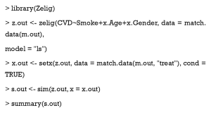
MatchIt does not provide functions for estimating treatment effects; however, Ho et al. (70) noted that any software for parametric statistical analyses may be used to analyze data previously preprocessed by MatchIt. They provided an example where they used the Zelig package to estimate treatment effects. Keller and Tipton (77) observed errors when they ran certain versions (4.2-1) of the Zelig package; thus, researchers should check the versions of their R packages before performing the PSM analysis.
The Zelig package estimates causal effects from Monte Carlo simulations, which is beyond the scope of this tutorial. Herein, we provide an analogous example; readers are directed to the Zelig official document.
Other packages
Other models may also be used to estimate treatment effects. If 1:1 matching without replacement is implemented, the weights of each sample =1, and thus, the model does not require adjustment. However, the weighted versions of a specified model should be used, if the sample weights are ≠1. This is an example of weighted logistic regression.
Here the coefficient for smoking was 5.11, which means that for a patient in the treatment group, smoking behavior increased the risk for CVD (before the logistic transform) by 5.11 points.
What about unmeasured covariates related to treatment allocation and outcomes?
Sensitivity analysis
Although PSM balances data based on covariates, there may still be some confounding factors that have not been collected in the dataset, which may introduce hidden bias to the study (8). A core advantage of a well-implemented RCT is that it reduces as much as possible both obvious and hidden biases, while in observational studies, PSM and other analogous methods can only balance data based on recorded covariates.
Sensitivity analyses of observational studies help analyze the influence of unobserved confounders on the results (78). The origins of the approach can be traced back to a dispute on the relationship between smoking and lung cancer (79). It appears that no matter how many more smokers get lung cancer when compared to those who do not, champions of smoking argue for certain unobserved confounders, for example, genetic make-up related to both smoking behavior and risk of cancer. Therefore, it is necessary to measure the influence of hidden covariates on research in order to obtain even more convincing conclusions. In this section, we introduce three representative methods to deal with hidden biases.
From the perspective of statistical testing, Rosenbaum’s sensitivity analysis (55) finds a influence threshold in a study. When the influence of unobserved confounders on the study exceeds the threshold, our conclusion, based only on observed covariates, is insignificant. In other words, when the hidden bias is small, our conclusions are still valid, but when the hidden bias is much larger, they can be questioned. Actually, Rosenbaum’s sensitivity analysis evaluates how sensitive a study is to hidden bias, and is frequently used after PSM (78). This method has now been developed into primal, dual, and simultaneous analyses. Their differences are based on what associations between unobserved confounders and the study are analyzed (80). In short, primal analysis focuses on associations between unobserved confounders and treatment assignments, dual analysis centers on associations between unobserved confounders and outcome, and simultaneous analysis accounts for both.
Here, we introduce what primal analysis is and how to implement it with an R package called rbounds. Suppose there are two patients, Bob and Bill. In a perfect study free of hidden bias, as long as Bob and Bill have the same observed covariates X, then they have the same probability of receiving treatment. Yet, if there is a hidden bias, even though Bob and Bill have the same X, their probabilities of receiving treatment are different, due to these different unobserved covariates. Thus, the boundary of the odds ratio (OR) of their probabilities of receiving treatment measures the degree of departure from a study that is free of hidden bias. That is to say, when the hidden bias in a study is greater, the treatment probabilities of patients with the same observed covariates are more different, and the deviation of the OR from 1 will be greater.
Primal sensitivity analysis sets as the boundary of OR and tests the validity of the conclusions with various levels. When becomes larger, the relationship between hidden bias and treatment assignment grows stronger. The analysis provides the confidence intervals of P values with each . The larger with upper bound of P value <0.05 is observed, the more robust the study conclusion is with hidden bias. The readers are referred to Guo and Fraser’s work (1) for further theoretical analysis.
However, the main disadvantage of Rosenbaum’s sensitivity analysis is that these methods are designed only for 1:1 matching (78,81), thereby substantially limiting the methodology.
Vanderweele and Arah (81) proposed a general method for sensitivity analysis, which allowed for binary, ordinal, or continuous outcomes; categorical or continuous treatment; and categorical or continuous observed and unobserved variables. They proved a set of bias formulas which can be used to estimate the bias factor and obtain the true OR of the relationship between treatment and outcomes. However, if these formulas are applied, simplifying assumptions must be made based on knowledge or external data, and the specification of sensitivity parameters in the formulas. Liu et al. (78) introduced and summarized Rosenbaum’s and Vanderweele and Arah’s methods. Interested readers are directed to their article (78).
After this, Vanderweele further explored sensitivity analysis without assumptions, and introduced the E value (82,83). E value is defined as the minimum strength of association, on the risk ratio scale, that an unmeasured confounder must have with both the treatment and the outcome, conditional on the measured covariates, to fully explain away a specific treatment–outcome association. Although it is similar to Rosenbaum’s methods, the E value makes no assumptions on whether unmeasured confounders are binary, continuous, or categorical. It makes no assumptions on how they are distributed, or on the number of confounders, and it can be applied to several common outcome types in observational research studies. To facilitate these sensitivity analyses, Mathur et al. provided an R package (“EValue”) and an online E value calculator (https://mmathur.shinyapps.io/evalue/) (84).
Propensity score calibration (PSC) is another method that deals with hidden bias, and is similar to regression calibration (85). For example, if you study the effects of norepinephrine on mortality using PSM, you may already have a large dataset to support your research; however, you may speculate that central venous pressure (CVP) is a potential confounding variable, but it is not measured in your dataset. In this case, another small dataset, containing CVP and all covariates in the large dataset, can be collected. The steps of PSC are as follows: (I) estimate raw PS in your main dataset; (II) estimate PS in your validation dataset with the same set of covariates as the main one (denoted as PS1), and with an extended covariate set including CVP as PS2; (III) model the extended PS2 as a function of PS1; and (IV) calibrate your raw PS on the main dataset, with the function mentioned above (III).
How to implement sensitivity analysis with R
In this section, we show how to implement sensitivity analysis using R. Our treatment assignment and outcomes were related to gender and patient age, while here we use only age to estimate PS, and gender is the unobserved confounding variable. There are no missing values in our data. We divided our data into two datasets, using an 8:2 ratio to implement the PSC. Note that to simplify our tutorial, we did not balance the covariates, which is not permitted in actual research.
Rosenbaum’s primal sensitivity analysis
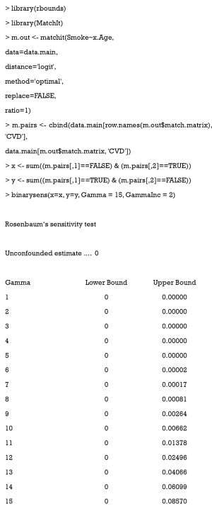
The R package rbounds provides functions to implement Rosenbaum’s sensitivity analysis for binary, continuous, or ordinal outcomes. First, this package must be installed and uploaded. The package directly analyzes the match object from the Matching package. Because we used MatchIt to implement PSM, we must obtain matched outcomes prior to running the functions of rbounds, using the following code:
match.matrix records the matching relationship between the treatment and control groups. The cbind function generates a matrix where the first column is the treated outcomes, and the second column is the controlled outcomes.
In the rbounds package, the functions, binarysens and psens are commonly used. The former is used for binary outcomes, and the latter for continuous or ordinal outcomes. Here, we used binarysens. This function has four arguments: x, y, Gamma, and GammaInc. The argument x is the number of pairs where the controlled patients have outcomes, but the treated patients do not. The argument y is the number of pairs where the treated patients have outcomes, but the controlled patients do not. The argument Gamma is the maximum tested in our study. The argument GammaInc is the step size of , when it changes from small to large. We must count the number of discordant pairs, followed by the function, binarysens.
Here, the value of x is 4 while that of y is 126. The first column represents the different values of Gamma , while the second and third are the lower and upper bound of the P value, respectively. This P value is calculated by testing whether or not our result is significant. Lower bounds are recorded as 0, because they are extremely small (<0.00001). As observed, the upper bound <0.05, when Gamma <14. This means that even if one patient may be 13 times as likely to be treated as another with the same recorded covariates, due to the hidden bias, the treatment still contributes significantly to the outcome.
If you need to manage continuous or ordinal outcomes, the following code can be run:
Here, x is the treatment group outcomes, while y is the control group outcomes.
E value
Firstly, the corresponding package must be installed and uploaded.
The evalue function is the core element of this package, which computes E values for unmeasured confounding factors. The argument est is the effect estimate that is observed but is suspected to be biased. The estimate can be a particular type of effect measure, e.g., risk ratio (RR), odds ratio (OR), hazard ratio (HR), risk difference (RD), linear regression coefficient (OLS), or mean standardized difference (MD). For example, if the RR estimate was 0.80 and the lower and upper bound were 0.70 and 0.90, respectively, then the E value would be calculated as follows:
This package is relatively simple, except for the explanation for E value. Interested readers are directed to the following website: https://cran.r-project.org/web/packages/EValue/EValue.pdf.
PSC
First, raw PS is estimated with our main data.
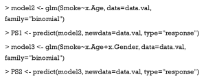
Second, PS1 is estimated with the same set of covariates on the validation data, and PS2 is estimated with gender being added.
Then, PS2 is regressed on PS1.
Finally, our raw PS is calibrated.
How does PSM handle multiple or continuous treatments?
The PS is the conditional probability of receiving treatment, given that covariates are observed. It effectively balances covariates between treatment and control groups, when the treatment assignment is dichotomous. However, on account of the complexity of medical research, researchers sometimes have to face comparisons of multiple treatments, or analyze the effects of different treatment doses (60,86,87). The original PS definition and related analytical methods are no longer applicable, and thus we must extend the concept of PS for more complex settings.
GPS for multiple treatments
Definitions
Now, we try to estimate and compare the effects of three different treatments: treatment A, B, and C (or control). Paired comparisons with PSM, which include separately applying PSM to A–B, A–C, and B–C, is a direct analytical method (60). However, because some patients are discarded during matching, the paired comparisons are actually based on different patient groups. Therefore, it is possible that a researcher using pairwise PSM observes that A is better than B, B is better than C, and C is better than A (86). Furthermore, when treatment numbers increase, there are squared-level number of pairs to analyze. Another way is to determine a reference treatment, e.g., C, then match A vs. C, and B vs. C (88,89). This is an ingenious method when the influence of treatment C is focused on in the study. However, the comparison of A and B is challenging in this study design.
Rassen et al. (90) proposed a three-way matching algorithm which can simultaneously match participants from 3 groups. This was based on GPS and online codes. Herein, we introduce GPS and show how to estimate GPS using multinomial logistic regression with R.
Conceptually, GPS is the probability that a patient receives 1 of several possible treatments, conditional on his or her covariates. It is usually estimated by multinomial logistic regression. This prediction model chooses 1 treatment (for example, C) as the baseline treatment (reference). Next, the logarithm of ratio of the probabilities of receiving treatment A (or B) and reference treatment is assessed for every patient. Lastly, the model provides a matrix of probabilities for each patient to receive each treatment. Equally, CART, random forests, and other machine learning methods can also predict the probability of receiving one treatment rather than the others (8,38). Currently, machine learning–augmented PS is a promising research area.
The estimation of GPS for multiple treatments with R
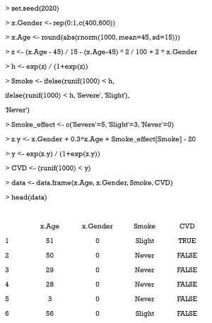
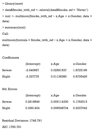
First, we must modify our dataset for multiple treatments. We group patients into three categories according to their smoking behavior—severe, slight, and never—and assume that older men are more prone to excessive smoking, and that increased smoking leads to a higher risk of CVD. The simulation data are generated with the following code:
Next, we choose the never-smoking group as a reference, and use the multinom function in the nnet package to estimate GPS.
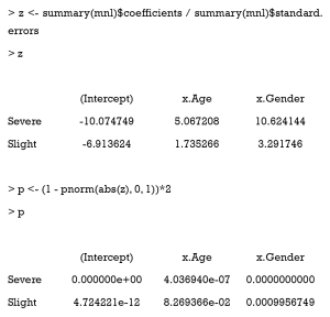
This function does not calculate P values for coefficients, but we can complete this ourselves.
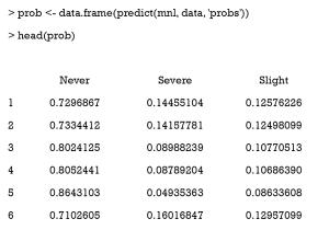
Then, we use the predict function to derive the probability of receiving one certain treatment. The mnl argument is the multinomial logistic regression model. The “probs” argument means the function returns a probability value (0–1) instead of the predicted class.
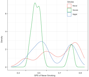
After this, we visualize the GPS distribution for different groups using the ggplot2 package. The following example is a density plot, which shows the GPS distribution of never smoking for different groups (Figure 11).
GPS for continuous treatments
Definitions
When we study the effects of various patient treatment dosages, the treatment assignment indicator is a continuous variable, e.g., the dosage of a new drug A. In a continuous setting, it is unlikely that two units will have exactly the same level of treatment, so it is unfeasible to match pairs with the same exposure level (91). Hirano and Imbens (92) proposed an extension to the counterfactual framework. In their approach, a set of potential outcomes for each patient is considered; however, only 1 value of the set is observed. Their method of estimating the effects of continuous treatments consists of three stages: (I) the treatment dose is regressed on a function of covariates with a linear regression model, assuming the residual is normally distributed, and the estimated GPS is the probability of the observed residual (such a description is not precise, but easy to understand); (II) the outcomes are modeled as a function of the treatment dose and GPS; and (III), for each level of treatment of interest, the GPS is estimated using the model in stage 1, and subsequently the average potential outcome is obtained using the model in stage 2. After the potential outcome for multiple different treatment doses is estimated, the dose-response function is obtained. In addition to this approach, a variety of methods have been proposed to estimate the dose-response function, based on GPS (68,92-95), but to the best of our knowledge, these methods are not based on matching. Wu et al. (91) proposed a one-to-M nearest neighbor caliper matching procedure with replacement. For each unit, the algorithm finds the m observed unit that is both close to its exposure level and the corresponding estimated GPS. They kindly provided an R package for implementing matching on GPS with continuous exposures. Readers can visit the website at https://github.com/wxwx1993/GPSmatching. Herein, we introduce GPS estimation with R.
Estimating GPS for continuous treatments with R
We extended our simulation data to study the effects of different durations of smoking on the cardiovascular system. Years of smoking for each patient were generated by the following code, with the risk of CVD being assumed to be proportional to the years of smoking (YOS).
Here, YOS is generated as the linear combination of age and gender, with a normally distributed residual.
First, the YOS linear regression model and covariates are fitted.
Then, the GPS is estimated by the normal distribution.
How to apply PSM with time-dependent covariates and treatments
In clinical settings, especially where variables are continuously monitored, the probability of receiving a treatment is based on the real-time value of variables. Treatment effects are usually dependent on when a patient receives a treatment. Although a binary indicator can be generated to indicate whether a patient is treated or not throughout their admission, this conventional method leads to biased estimated treatment effects (96), because it does not account for the time factor of treatment.
Time-dependent PSM helps analyze the true effects of treatment (97). First, time-dependent PS is estimated for each patient at every time point, using a Cox proportional hazards regression model on time-fixed and time-varying covariates. Then, simultaneous matching or sequential matching is applied to match patients based on time-dependent PSs. Lastly, Cox regression or other models for time-to-event analysis are applied to the matched data.
As implied by the name, simultaneous matching compares all possible combinations of matched pairs at once, and performs one matching for all patients. However, this method assumes little association between future covariates and current treatment decisions, because future covariate information may be disclosed during the matching process. In contrast, no information leaks are allowed in sequential matching. As shown in Figure 12, the entire time is divided into multiple, equally spaced intervals (e.g., 5). At each interval, patients treated at that time form the treatment group, while patients untreated until that time form the control group (even though they may receive treatment after that). From the first interval to the last, treated patients are matched to untreated patients, using optimal matching. Once matched, patients are removed from groups, and they do not participate in subsequent matching processes. Zhang et al. (96) developed the function TDPSM for time-dependent PSM, and they have shared their R code.
Discussion
As previously discussed, the two main advantages of PSM are dimension reduction and study design separation. Some conventional methods, for example, matching or stratification, group units with the same or similar covariate values to eliminate confounding. However, when covariate numbers increase, matching or stratification becomes much more difficult. Take research data on 1,000 patients as an example. To eliminate bias due to gender, each patient may be matched to 500 patients of the opposite gender. Also, if we consider age as a confounding factor, the data can be divided into 10 equal groups by age, after which each patient can be matched to about 50 others. Furthermore, race is accounted for, and thus for each patient only 10 are matched. If we keep adding balancing covariates, many patients will not be matched. When compared with matching or stratification, all covariates requiring balancing are integrated into 1 score in PSM. This integration greatly reduces matching difficulties due to covariate dimensions.
In addition, covariate balancing and effect estimating are separated in PSM. As Figure 2 illustrates, it is possible to check whether or not covariates are balanced between treatment and control groups in the fourth step, and estimate treatment effects later. In the regression adjustment method, which models outcomes as functions of both treatment assignments and covariates, it is difficult to assess whether the model has been correctly specified. Goodness-of-fit measures, such as R2 and MSE do not test whether the model has balanced the data or not (3).
While these advantages make PS methods popular, there are several limitations. Firstly, the greatest drawback to PS methods is that they cannot account for hidden bias, which is similar to other methods which derive causal inference from observational research. Most balancing methods can only adjust data based on recorded covariates. However, it is inevitable that there is unobservable, immeasurable, or unrecorded bias. Although sensitivity analyses evaluate study robustness or calibrate PS with validation datasets, there is still room for improvement. In contrast, in a well-structured RCT, obvious or hidden bias is reduced as much as possible, and therefore, PSM and analogous methods are no replacement for randomization. However, PSM can be used to scrutinize relationships between treatments and outcomes prior to the commencement of an RCT. On account of the limited medical resources, PSM and other balancing methods are still of great value.
Secondly, sample size is often diminished in PSM, as patients with no matches are often discarded. This may negatively affect final study conclusions, especially when small sample sizes are used. When several thousand samples are included, the data loss is negligible.
Thirdly, PSM estimates average treatment effects, but treatment heterogeneity is not considered. As we enter the era of precision medicine, personalized therapeutic strategies are being increasingly emphasized. However, personalized medicine is still a long way from being fully realized.
In this tutorial, we introduced the concept and framework of PSM, showed how to implement PSM with R, demonstrated GPS for multiple and continuous treatments, and illustrated time-dependent PSM. However, the statistical basics of PSM were not covered in this tutorial. Besides, there are many other R packages related to PS, and other methods based on PS, such as weighting or subclassification, which were not included in this tutorial. In light of the rapid growth of causal inference analysis in observational studies, more comprehensive tutorials on PS methods should be developed.
Acknowledgments
We thank International Science Editing (
Funding: This article was supported by grants from the Research Funds of Shanghai Municipal Health Commission (No. 2019ZB0105), Natural Science Foundation of Shanghai (No. 20ZR1411100), Program of Shanghai Academic/Technology Research Leader (No. 20XD1421000), National Natural Science Foundation of China (No. 82070085), Clinical Research Funds of Zhongshan Hospital (No. 2020ZSLC38 and No. 2020ZSLC27), and Smart Medical Care of Zhongshan Hospital (No. 2020ZHZS01).
Footnote
Conflicts of Interest: All authors have completed the ICMJE uniform disclosure form (available at http://dx.doi.org/10.21037/atm-20-3998). GWT served as an unpaid section editor of the Annals of Translational Medicine from October 2019 to September 2020. The other authors have no other conflicts of interest to declare
Ethical Statement: The authors are accountable for all aspects of the work in ensuring that questions related to the accuracy or integrity of any part of the work are appropriately investigated and resolved.
Open Access Statement: This is an Open Access article distributed in accordance with the Creative Commons Attribution-NonCommercial-NoDerivs 4.0 International License (CC BY-NC-ND 4.0), which permits the non-commercial replication and distribution of the article with the strict proviso that no changes or edits are made and the original work is properly cited (including links to both the formal publication through the relevant DOI and the license). See: https://creativecommons.org/licenses/by-nc-nd/4.0/.
1We indiscriminately used the terms propensity score and estimated propensity score. Guo and Fraser (1) summarized the meaning of these terms. In this tutorial, PS as estimated by our model, is called estimated propensity score, unless explicitly stated otherwise.
2We use the term “treatment” throughout this article to simplify the language, although it is sometimes better to use “exposure” or “intervention”.
References
- Guo S, Fraser MW. Propensity score analysis: Statistical methods and applications. SAGE Publications; 2014.
- Cook TD, Campbell DT, Shadish W. Experimental and quasi-experimental designs for generalized causal inference. Boston: Houghton Mifflin; 2002.
- Austin PC. An introduction to propensity score methods for reducing the effects of confounding in observational studies. Multivariate Behav Res 2011;46:399-424. [Crossref] [PubMed]
- Cochran WG, Chambers SP. The planning of observational studies of human populations. J R Stat Soc Ser A 1965;128:234-66. [Crossref]
- Tein JY, Mazza GL, Gunn HJ, et al. Multigroup propensity score approach to evaluating an effectiveness trial of the New Beginnings Program. Eval Health Prof 2018;41:290-320. [Crossref] [PubMed]
- Rosenbaum PR, Rubin DB. The central role of the propensity score in observational studies for causal effects. Biometrika 1983;70:41-55. [Crossref]
- Mitra R, Reiter JP. A comparison of two methods of estimating propensity scores after multiple imputation. Stat Methods Med Res 2016;25:188-204. [Crossref] [PubMed]
- Leite W. Practical propensity score methods using R. SAGE Publications; 2016.
- Randolph JJ, Falbe K, Manuel AK, et al. A step-by-step guide to propensity score matching in R. Pract Assess Res Eval 2014;19:18.
- Zhang Z. Propensity score method: a non-parametric technique to reduce model dependence. Ann Transl Med 2017;5:7. [Crossref] [PubMed]
- Zhang Z, Kim HJ, Lonjon G, et al. Balance diagnostics after propensity score matching. Ann Transl Med 2019;7:16. [Crossref] [PubMed]
- Yao XI, Wang X, Speicher PJ, et al. Reporting and guidelines in propensity score analysis: a systematic review of cancer and cancer surgical studies. J Natl Cancer Inst 2017;109:djw323 [Crossref] [PubMed]
- Malla L, Pererasalazar R, Mcfadden E, et al. Handling missing data in propensity score estimation in comparative effectiveness evaluations: a systematic review. J Comp Eff Res 2018;7:271-9. [Crossref] [PubMed]
- Zakrison TL, Austin P, McCredie V. A systematic review of propensity score methods in the acute care surgery literature: avoiding the pitfalls and proposing a set of reporting guidelines. Eur J Trauma Emerg Surg 2018;44:385-95. [Crossref] [PubMed]
- Austin PC. Type I error rates, coverage of confidence intervals, and variance estimation in propensity-score matched analyses. Int J Biostat 2009;5:13 [Crossref] [PubMed]
- Austin PC, Grootendorst P, Anderson GM. A comparison of the ability of different propensity score models to balance measured variables between treated and untreated subjects: a Monte Carlo study. Stat Med 2007;26:734-53. [Crossref] [PubMed]
- Austin PC, Mamdani MM. A comparison of propensity score methods: a case‐study estimating the effectiveness of post‐AMI statin use. Stat Med 2006;25:2084-106. [Crossref] [PubMed]
- Rubin DB. On principles for modeling propensity scores in medical research. Pharmacoepidemiol Drug Saf 2004;13:855-7. [Crossref] [PubMed]
- Huang F, Du C, Sun M, et al. Propensity score matching in SPSS. Nan Fang Yi Ke Da Xue Xue Bao 2015;35:1597-601. [PubMed]
- Enders CK. Applied missing data analysis. Guilford Press; 2010.
- Zhang Z. Missing data imputation: focusing on single imputation. Ann Transl Med 2016;4:9. [PubMed]
- Groenwold RHH, White IR, Donders ART, et al. Missing covariate data in clinical research: when and when not to use the missing-indicator method for analysis. CMAJ 2012;184:1265-9. [Crossref] [PubMed]
- Malarvizhi R, Thanamani AS. K-nearest neighbor in missing data imputation. Int J Eng Res Dev 2012;5:5-7.
- Pantanowitz A, Marwala T. Missing data imputation through the use of the Random Forest Algorithm. Advances in Computational Intelligence. Springer; 2009: 53-62.
- Tang F, Ishwaran H. Random forest missing data algorithms. Stat Anal Data Min 2017;10:363-77. [Crossref] [PubMed]
- Leyrat C, Seaman SR, White IR, et al. Propensity score analysis with partially observed covariates: How should multiple imputation be used? Stat Methods Med Res 2019;28:3-19. [Crossref] [PubMed]
- Stuart EA. Matching methods for causal inference: A review and a look forward. Stat Sci 2010;25:1-21. [Crossref] [PubMed]
- Leite W, Aydin B. editors. A comparison of methods for imputation of missing covariate data prior to propensity score analysis. Washington, DC: American Education Research Association Conference, 2016.
- Choi J, Dekkers OM, Cessie SL. A comparison of different methods to handle missing data in the context of propensity score analysis. Eur J Epidemiol 2019;34:23-36. [Crossref] [PubMed]
- Puma M, Olsen RB, Bell SH, et al. What to Do when Data Are Missing in Group Randomized Controlled Trials. NCEE 2009:0049.
- Lee BK, Lessler J, Stuart EA. Improving propensity score weighting using machine learning. Stat Med 2010;29:337-46. [Crossref] [PubMed]
- Pearl J. Causal diagrams for empirical research. Biometrika 1995;82:669-88. [Crossref]
- Pearl J, Mackenzie D. The book of why: the new science of cause and effect. Basic Books; 2018.
- Brookhart MA, Schneeweiss S, Rothman KJ, et al. Variable selection for propensity score models. Am J Epidemiol 2006;163:1149-56. [Crossref] [PubMed]
- Cuong NNV. Which covariates should be controlled in propensity score matching? Evidence from a simulation study. Stat Neerl 2013;67:169-80. [Crossref]
- Gottesman O, Johansson F, Komorowski M, et al. Guidelines for reinforcement learning in healthcare. Nat Med 2019;25:16-8. [Crossref] [PubMed]
- McCaffrey DF, Ridgeway G, Morral AR. Propensity Score Estimation with Boosted Regression for Evaluating Causal Effects in Observational Studies. Psychol Methods 2004;9:403-25. [Crossref] [PubMed]
- McCaffrey DF, Griffin BA, Almirall D, et al. A Tutorial on Propensity Score Estimation for Multiple Treatments Using Generalized Boosted Models. Stat Med 2013;32:3388-414. [Crossref] [PubMed]
- Setoguchi S, Schneeweiss S, Brookhart MA, et al. Evaluating uses of data mining techniques in propensity score estimation: a simulation study. Pharmacoepidemiol Drug Saf 2008;17:546-55. [Crossref] [PubMed]
- Keller B, Kim J, Steiner PM. Propensity Score Estimation with Data Mining Techniques: Alternatives to Logistic Regression. Soc Res Educ Effectiveness 2013.
- Keller BS, Kim J-S, Steiner PM. Data mining alternatives to logistic regression for propensity score estimation: Neural networks and support vector machines. Multivariate Behav Res 2013;48:164. [Crossref] [PubMed]
- Westreich D, Lessler J, Funk MJ. Propensity score estimation: neural networks, support vector machines, decision trees (CART), and meta-classifiers as alternatives to logistic regression. J Clin Epidemiol 2010;63:826-33. [Crossref] [PubMed]
- De Vries BBLP, Van Smeden M, Groenwold RHH. Propensity score estimation using classification and regression trees in the presence of missing covariate data. Epidemiol Methods 2018;7.
- Wyss R, Schneeweiss S, Der Laan MJV, et al. Using Super Learner Prediction Modeling to Improve High-dimensional Propensity Score Estimation. Epidemiology 2018;29:96-106. [Crossref] [PubMed]
- Rubin DB. Bias Reduction Using Mahalanobis-Metric Matching. Biometrics 1980;36:293. [Crossref]
- Cochran WG, Rubin DB. Controlling bias in observational studies: A review. Indian J Stat Ser A 1973;417-46.
- Rosenbaum PR, Rubin DB. Constructing a Control Group Using Multivariate Matched Sampling Methods That Incorporate the Propensity Score. Am Stat 1985;39:33-8.
- Austin PC. A comparison of 12 algorithms for matching on the propensity score. Stat Med 2014;33:1057-69. [Crossref] [PubMed]
- Rosenbaum PR. Optimal Matching for Observational Studies. J Am Stat Assoc 1989;84:1024-32. [Crossref]
- Bertsekas DP. Linear network optimization: algorithms and codes. MIT Press; 1991.
- Hansen BB. Optmatch: Flexible, optimal matching for observational studies. N Funct Multivariate Anal 2007;7:18-24.
- Gu XS, Rosenbaum PR. Comparison of Multivariate Matching Methods: Structures, Distances, and Algorithms. J Comput Graph Stat 1993;2:405-20.
- Diamond A, Sekhon JS. Genetic Matching for Estimating Causal Effects: A General Multivariate Matching Method for Achieving Balance in Observational Studies. Rev Econ Stat 2013;95:932-45. [Crossref]
- Hansen BB. Full matching in an observational study of coaching for the SAT. J Am Stat Assoc 2004;99:609-18. [Crossref]
- Rosenbaum P. Observational Studies (2nd ed.). New York: Springer, 2002.
- Austin PC. Optimal caliper widths for propensity-score matching when estimating differences in means and differences in proportions in observational studies. Pharm Stat 2011;10:150-61. [Crossref] [PubMed]
- Rubin DB. Using Propensity Scores to Help Design Observational Studies: Application to the Tobacco Litigation. Health Serv Outcomes Res Methodol 2001;2:169-88. [Crossref]
- Lan P, Wang T, Li H, et al. Utilization of echocardiography during septic shock was associated with a decreased 28-day mortality: a propensity score-matched analysis of the MIMIC-III database. Ann Transl Med 2019;7:662. [Crossref] [PubMed]
- Zhang Z, Zhu C, Mo L, et al. Effectiveness of sodium bicarbonate infusion on mortality in septic patients with metabolic acidosis. Intensive Care Med 2018;44:1888-95. [Crossref] [PubMed]
- Zeng C, Dubreuil M, Larochelle MR, et al. Association of Tramadol With All-Cause Mortality Among Patients With Osteoarthritis. JAMA 2019;321:969-82. [Crossref] [PubMed]
- Imai K, King G, Stuart EA. Misunderstandings between experimentalists and observationalists about causal inference. J R Stat Soc Ser A Stat Soc 2008;171:481-502. [Crossref]
- Austin PC. A critical appraisal of propensity‐score matching in the medical literature between 1996 and 2003. Stat Med 2008;27:2037-49. [Crossref] [PubMed]
- Austin PC. The Relative Ability of Different Propensity Score Methods to Balance Measured Covariates Between Treated and Untreated Subjects in Observational Studies. Med Decis Making 2009;29:661-77. [Crossref] [PubMed]
- Deb S, Austin PC, Tu JV, et al. A Review of Propensity-Score Methods and Their Use in Cardiovascular Research. Can J Cardiol 2016;32:259-65. [Crossref] [PubMed]
- Rubin DB. Estimating Causal Effects of Treatments in Randomized and Nonrandomized Studies. J Educ Psychol 1974;66:688-701. [Crossref]
- Abadie A, Imbens GW. Simple and bias-corrected matching estimators for average treatment effects: National Bureau of Economic Research2002. Report No.: 0898-2937.
- Abadie A, Imbens GW. Large sample properties of matching estimators for average treatment effects. Econometrica 2006;74:235-67. [Crossref]
- Imbens GW. The Role of the Propensity Score in Estimating Dose-Response Functions. Biometrika 1999;87:706-10. [Crossref]
- West SG, Cham H, Thoemmes F, et al. Propensity scores as a basis for equating groups: Basic principles and application in clinical treatment outcome research. J Consult Clin Psychol 2014;82:906-19. [Crossref] [PubMed]
- Ho DE, Imai K, King G, et al. MatchIt: Nonparametric preprocessing for parametric causal inference. J Stat Softw 2011;42:1-28. [Crossref]
- Neugebauer R. Laan Mvd. Why prefer double robust estimators in causal inference? J Stat Plan Inference ;129:405-26. [Crossref]
- Schafer JL, Kang J. Average causal effects from nonrandomized studies: a practical guide and simulated example. Psychol Methods 2008;13:279. [Crossref] [PubMed]
- Rubin DB. Causal Inference Using Potential Outcomes: Design, Modeling, Decisions. J Am Stat Assoc 2005;100:322-31. [Crossref]
- Rubin DB. The design versus the analysis of observational studies for causal effects: parallels with the design of randomized trials. Stat Med 2007;26:20-36. [Crossref] [PubMed]
- Rubin DB. For objective causal inference, design trumps analysis. Ann Appl Stat 2008;2:808-40. [Crossref]
- Austin PC. Comparing paired vs non‐paired statistical methods of analyses when making inferences about absolute risk reductions in propensity‐score matched samples. Stat Med 2011;30:1292-301. [Crossref] [PubMed]
- Keller B, Tipton E. Propensity Score Analysis in R: A Software Review. J Educ Behav Stat 2016;41:326-48. [Crossref]
- Liu W, Kuramoto SJ, Stuart EA. An introduction to sensitivity analysis for unobserved confounding in nonexperimental prevention research. Prev Sci 2013;14:570-80. [Crossref] [PubMed]
- Cornfield J, Haenszel W, Hammond EC, et al. Smoking and lung cancer: recent evidence and a discussion of some questions. J Natl Cancer Inst 1959;22:173-203. [PubMed]
- Gastwirth JL, Krieger AM, Rosenbaum PR. Dual and simultaneous sensitivity analysis for matched pairs. Biometrika 1998;85:907-20. [Crossref]
- Vanderweele TJ, Arah OA. Bias formulas for sensitivity analysis of unmeasured confounding for general outcomes, treatments, and confounders. Epidemiology 2011;22:42-52. [Crossref] [PubMed]
- Ding P, Vanderweele TJ. Sensitivity Analysis Without Assumptions. Epidemiology 2016;27:368-77. [Crossref] [PubMed]
- VanderWeele TJ, Ding P. Sensitivity Analysis in Observational Research: Introducing the E-Value. Ann Intern Med 2017;167:268-74. [Crossref] [PubMed]
- Mathur MB, Ding P, Riddell CA, et al. Website and R package for computing E-values. Epidemiology 2018;29:e45 [Crossref] [PubMed]
- Spiegelman D, Mcdermott A, Rosner B. Regression calibration method for correcting measurement-error bias in nutritional epidemiology. Am J Clin Nutr 1997;65:1179S-86S. [Crossref] [PubMed]
- Cui ZL, Hess LM, Goodloe R, et al. Application and comparison of generalized propensity score matching versus pairwise propensity score matching. J Comp Eff Res 2018;7:923-34. [Crossref] [PubMed]
- Wang Y, Cai H, Li C, et al. Optimal caliper width for propensity score matching of three treatment groups: a Monte Carlo study. PLoS One 2013;8:e81045 [Crossref] [PubMed]
- Solomon DH, Rassen JA, Glynn RJ, et al. The Comparative Safety of Analgesics in Older Adults With Arthritis. JAMA Intern Med 2010;170:1968-78. [Crossref] [PubMed]
- Solomon DH, Rassen JA, Glynn RJ, et al. The Comparative Safety of Opioids for Nonmalignant Pain in Older Adults. JAMA Intern Med 2010;170:1979-86. [Crossref] [PubMed]
- Rassen JA, Shelat A, Franklin JM, et al. Matching by Propensity Score in Cohort Studies with Three Treatment Groups. Epidemiology 2013;24:401-9. [Crossref] [PubMed]
- Wu X, Mealli F, Kioumourtzoglou M, et al. Matching on Generalized Propensity Scores with Continuous Exposures. arXiv:181206575v3 [Preprint] 2018 [cited 2020 Jul 14].
- Hirano K, Imbens GW. The Propensity Score with Continuous Treatments. John Wiley & Sons, Ltd; 2005.
- Yang W, Joffe MM, Hennessy S, et al. Covariance Adjustment on Propensity Parameters for Continuous Treatment in Linear Models. Stat Med 2014;33:4577-89. [Crossref] [PubMed]
- Zhang Z, Zhou J, Cao W, et al. Causal inference with a quantitative exposure. Stat Methods Med Res 2016;25:315-35. [Crossref] [PubMed]
- Bia M, Mattei A. A Stata package for the estimation of the dose–response function through adjustment for the generalized propensity score. Stata J 2008;8:354-73. [Crossref]
- Zhang Z, Li X, Wu X, et al. Propensity score analysis for time-dependent exposure. Ann Transl Med 2020;8:246. [Crossref] [PubMed]
- Lu B. Propensity score matching with time-dependent covariates. Biometrics 2005;61:721-8. [Crossref] [PubMed]
(English Language Editor: J. Jones; Quality Control Editor: J. Gray)


