Multiple imputation for time series data with Amelia package
Introduction
Time series data are frequently encountered in medical research (1,2). In such dataset, individuals are measured for a particular variable repeatedly over time. For example, during general anesthesia patients may have their blood pressure and heart rate recorded every 5 min. A study comparing analgesic efficacy of two analgesics may use the blood pressure and heart rate as study end point. There are varieties of terms for such time series data in the literature. In politics and economics, investigators call them time series cross sectional data (3,4). In psychology, researchers follow participants for their developmental trends across life span and called this longitudinal study (or longitudinal survey). Despite of disparity in terminology, one important feature of such data is that time series values usually progress smoothly over time, and conventional multiple imputation (MI) algorithm fails to take this into consideration. Recall that we have previously used imputation() function from longitudinalData package for single imputation for longitudinal data. However, single imputation fails to consider imputation uncertainty and usually underestimates the variance. This article provides a step-by-step tutorial on how to perform MI for time series data. Some basic ideas behind the algorithms are provided. Interested readers are referred to references for more details on mathematical equations.
Basic ideas behind Amelia package
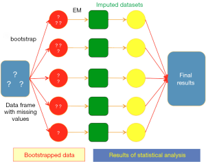
Bootstrap-based EM algorithm is employed to impute missing values. The algorithm draws m (the number of imputation dataset) samples of size n (the size of original dataset) from original dataset. Point estimates of mean and variance (both are vectors) are performed in each sample by using EM method. Remember there are m sets of estimates. Then each set of estimates is used to impute the missing observations from original dataset. The result is m sets of imputed data that can be used for subsequent analyses (Figure 1). Detailed description of bootstrap-based EM algorithm may be too complex for non-statistician readers and readers can refer to the chapter (4) if they need more detailed descriptions.
By assuming that time series data vary smoothly over time, observed values close in time to the missing value can greatly aid imputation of that value. However, the trend pattern may vary over time. A patient may experience sustained hypotension and lactate raises rapidly. Then after adequate resuscitation, he or she may recover from shock and lactate drops. In different situations observed values would be used in different way to impute missing values. One advantage of Amelia is able to incorporate polynomials of time to fit a model to predict missing values. In the following example I will show the difference in imputations with and without polynomials of time.
Working example
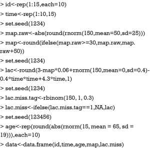
For hemodynamically unstable patients, mean blood pressure (map) and serum lactate (lac) are measured on daily basis. The latter is a reflection of tissue perfusion, and high lac values are the result of hypotension and tissue hypoperfusion. I created 15 patients and each one is followed up for 10 days.
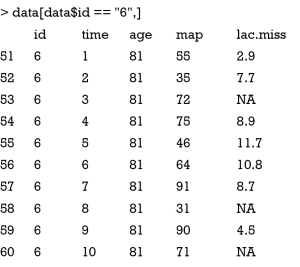
The id variable repeated for 10 times for each patient, and each measurement time is denoted by time variable from 1 to 10. Mean blood pressure (map) is simulated by assuming a normal distribution with a mean of 50 and a standard deviation of 25. An arbitrary value of 50 is added to map values less than 30. Lactate (lac) is the function of map and time. Higher map is associated with lower values of lac. Furthermore, lac follows a natural disease progression pattern, which goes up at the initial phase (disease progression), reaches a plateau and then returns to normal range thereafter. It is like a quadratic function with negative coefficient for the quadratic term. There is an uncertainty in lac values that cannot be accounted for by either map or time. Roughly 30% of lac values are missing, and the missing pattern is missing completely at random (MCAR). The variable age assumes a normal distribution and one patient has a fixed age value (e.g., age does not change within ten days). Lastly, simulated variables are aggregated within a data frame.
Multiple imputation (MI)
MI with amelia() function can be simply performed by the following code (5).
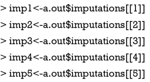
The first argument assigns a data frame with missing values to the Amelia() function. The number of imputed datasets to create is defined by m. In this function, the effect of time is not incorporated into the model. The imputed datasets can be visited by the following code. Because there are five imputed datasets, I create five data frame objects and each contains the imputed dataset.
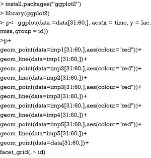
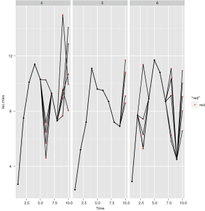
It would be interesting to visualize the imputed data in each individual. For the purpose of visualization of time series data, you may use the ggplot2 package (6). The graphical grammar of this package is based on the Grammar of Graphics (7). ggplot2 works in a layered fashion, starting with a layer showing the raw data then adding layers of additional symbols. In the example, longitudinal trends of imputed datasets are drawn layer after layer.
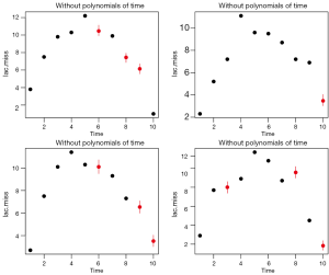
Figure 2 shows the imputed values (red dot) and observed values (black dot). Each panel represents one individual patient. Here I arbitrary present the patient 3, 4 and 5. Note that the imputed data distributed across a wide range, suggesting a remarkable uncertainty, and the time trend in lac variation is not taken into consideration.
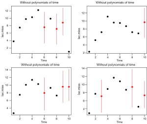
Otherwise, the imputed values can be visualized by using tscsPlot() function shipped with Amelia package (Figure 3).
Incorporating polynomials of time
Next, I will show how to incorporate the variable time into imputation.
As you can see, polynomials of time is assigned by the argument “polytime=2”. A polynomial power between 0 and 3 is allowed to account for the effects of time on variation of variable of interest. Other settings are the same to the above. Next, I would like to visualize the result of imputation when polynomials of time are incorporated into the model.
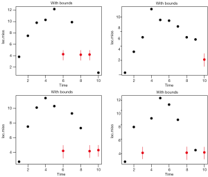
Figure 4 displays the same individuals as shown in Figure 3. Red dot and line represent posterior distribution of imputed values. Note that the distribution of imputed values is much more aggregated, suggesting more certainty in imputed values after incorporating of the time polynomials.
Lags and leads
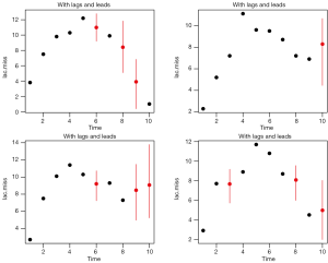
An alternative to take time into account is to use lags and leads of a variable. In Amelia package, lags are to take the value of another variable in the previous time, and leads are to take the value of another variable in the next time point. This task can be done by simply assign arguments to “lags=” and “leads=”. Note this assignment will take longer chain lengths.
The results are shown in Figure 5. As compared to Figure 4, the imputed values distributed more widely. However, the imputation is more influenced by lags and leads and the distribution appears better than Figure 3.
Prior information
Occasionally, investigators may have prior knowledge on the missing values based on previous published observations, academic consensus, and personal experience. When these are available, incorporation of such external information into imputation would greatly reduce uncertainty on imputations. The prior information can be used within the Bayesian framework. With Amelia package, prior information can be readily used by “priors=” argument. This argument receives a four or five column prior matrix.
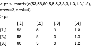
Supposed that I have prior information on lactate levels for the 6th patient. The mean lactate value is 3 because he survives the episode of shock and literature shows that patients with a mean lactate level of 3 are very likely to survive. However, there is uncertainty on this mean lac and a standard deviation of 1.2 is added. The prior matrix can be created by the following codes.
The first column is the row number of the missing values. The second column indicates the number of column of the variable with missing values. Third column contains the presumed mean of each missing values and the forth column is the standard deviation. With the prior matrix, MI can be performed with Amelia.
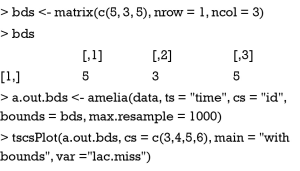
External information can also be used by logical bounds. Amelia can take draws from a truncated distribution, and the truncation is performed by setting bounds. In the example, suppose that you are certain that the missing values of the 6th patient fall between 3 and 5. Firstly, you need to create a bound matrix. Then the bound matrix can be passed to Amelia() function.
The results are shown in Figure 6. Note that the imputed values are restricted to the bound between 3 and 5.
Imputation diagnostics
Like diagnostics for regression model, imputed values also need to be checked for their plausibility. Amelia package provides several methods for diagnostics of imputation. You may compare distributions of imputed and observed values with following codes.
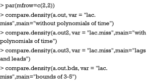
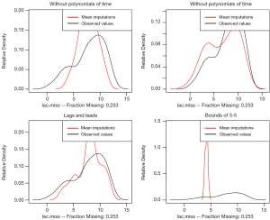
The par() function is to set graphical parameters. The “mfrow= c(2,2)” argument dictates that subsequent figures will be drawn in an 2-by-2 array. Compare.density() function is used to draw distributions of imputed and observed values (Figure 7). The results show that imputation with polynomials of time fits the best. Imputation with arbitrary bounds fits poorly. Another way to examine the imputation model is over-imputation.
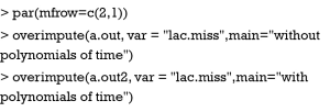
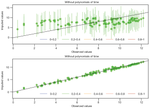
Over-imputation is a technique designed to test the fitness of imputation model. Each observed value is assumed to be missing, and imputed by using the imputation model. The horizontal line displays the actual observed value, and the vertical line denotes the imputed value pretending that the observed values are missing. The dots are mean value of imputation and lines represent 90% confidence interval. If mean values are on the diagonal line, the imputation model is exactly accurate. It is obvious from Figure 8 that imputation model with polynomials of time predicts well for missing values. The color of the line (in the bottom legend) shows the fraction of missing values in the missing pattern for that patient.
Summary
The article illustrates how to perform MI by using Amelia package in a clinical scenario. Amelia package is powerful in that it allows for MI for time series data. External information based on previous published observations, academic consensus, and personal experience can be incorporated by using prior or bound arguments. Diagnostics of imputation model can be performed by examining the distributions of imputed and observed values, or by using over-imputation technique.
Acknowledgements
None.
Footnote
Conflicts of Interest: The author has no conflicts of interest to declare.
References
- Chen B, Sumi A, Toyoda S, et al. Time series analysis of reported cases of hand, foot, and mouth disease from 2010 to 2013 in Wuhan, China. BMC Infect Dis 2015;15:495. [PubMed]
- Kennedy CE, Aoki N, Mariscalco M, et al. Using Time Series Analysis to Predict Cardiac Arrest in a PICU. Pediatr Crit Care Med 2015;16:e332-9. [PubMed]
- Beck N, Katz JN, Tucker R. Taking Time Seriously: Time-Series-Cross-Section Analysis with a Binary Dependent Variable. American Journal of Political Science 1998;42:1260-88.
- Honaker J, King G. What to Do about Missing Values in Time-Series Cross-Section Data. American Journal of Political Science. American Journal of Political Science 2010;54:561-81.
- Honaker J, King G, Blackwell M., Amelia II. A program for missing data. Journal of Statistical Software. 2011;45:1-47.
- Wickham H. ggplot2: elegant graphics for data analysis. New York: Springer-Verlag, 2009.
- Wilkinson L. The grammar of graphics. New York: Springer-Verlag, 2012.


