Reshaping and aggregating data: an introduction to reshape package

Introduction

In clinical studies involving data management of electronic medical record, variables are frequently grouped by one or more other variables (1). For example, when you follow up stroke patients for their quality of life (measured by some certain scores), the scores are recorded at each visit. In other words, these scores are nested within each patient. The display of such data can adopt long or wide format. The former listed each visit score longitudinally in a column and a variable denoting patient identification is mandatory. One patient can take up several rows in long format. One the other hand, the wide format displays 1 patient per row, and each visit score is listed consecutively in a single row. Both formats have their advantages and disadvantages depending on the purpose of analysis. These are a simple example illustrating the importance of data shape during analysis, and some are far more complex. This article introduces a powerful R package named “reshape”, which is able to handle varieties of data format (2).

Working example

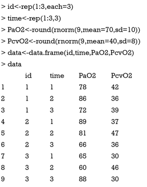
Suppose we have 3 patients, and each of them has blood partial pressure of oxygen measured on daily basis for 3 days. Blood oxygen can be measured from arterial line (PaO2) and central venous line (PcvO2).

Oxygen content is significantly lower in central vein than that in artery, which is consistent with the common sense that arterial oxygenation is much greater than venous oxygenation.

Melting a dataset

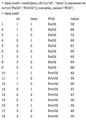
The melt() function converts a wide format into long format. A number of variables listed in columns can be stacked into a single column. As in our example, both venous and arterial partial pressures can be stacked in a single column after application of melt(). This function requires an id variable and variables of interests to be stacked. The generic form of melt() function is like this:

If either id.vars or measure.vars is specified, the function takes the remainder variable in the data frame belong to the other. If neither is specified, the function assumes the character and factor variable as the id.vars, and the remainders are measure.vars. To avoid confusion, you’d better specify both of them. The “variable_name” argument specified the name of the new variable that will be created to store stacked variables. Now let’s take a close look at how melt() works by using our working example.

Both id and time are id.vars and thus they remain unchanged. PaO2 and PcvO2 are stacked into a single column and a new variable called “PO2” is added to distinguish between arterial and venous oxygen. This melted format is not only useful for statistical analysis but also helpful in reshaping and aggregating data.

Casting a data frame

The cast() function contained in reshape package works on melted dataset. It transforms long data into wide format and can aggregate variable within any combinations of id variables. The generic form of cast() function takes the following form:

the argument data is a melted dataset. The cast formula has the format:

The x variables in combination define the rows, and y variables in combination defines the columns. If a set of x variables does not uniquely identify a row, the fun.aggregate argument should be given. Then the aggregate function can be applied to rows identified by a certain combination of x variables. List variables and z variables are usually not required. We don’t have dataset of that complex! Next, I will show how to cast the melted data in different formats.

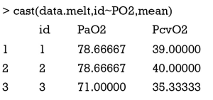
The rows are defined by the id variable on the left side of the formula, and columns are defined by PO2 variable. There are 2 levels contained in the PO2, thus we obtain 2 columns. Because the id variable does not uniquely identify a row, function mean is applied to vectors identified by id variable.

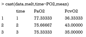
When id is replaced by time, the row represents mean value across id variable.

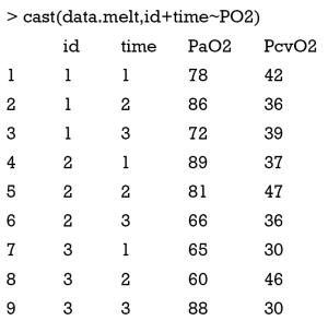
Variables id+time on the left side of the formula define the rows. Each unique combination of id and time defines a row. Columns are in line with the levels of PO2 variable. Because the 3 variables have identified a unique row, aggregating function is no longer applicable.

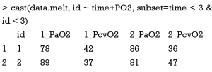
Data can be subset before reshaping. In the above example, we restrict subset of data with time<3 and id<3.

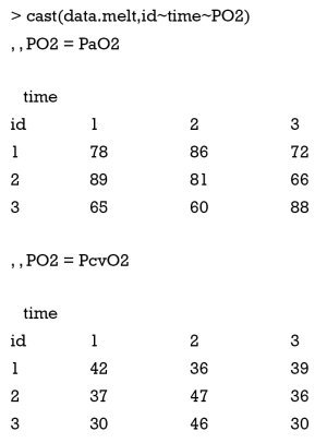
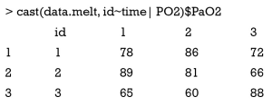
When a z variable is applied, we can see that the melted data is split into 2 datasets by variable PO2. Each item can be directly called by using the following code:

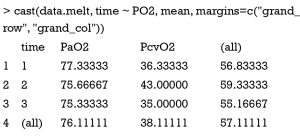
Row and column margins can be calculated with following code.

Split character vector into multiple columns

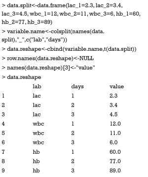
The function colsplit() in reshape package is to split character vector into multiple columns on certain expression. This can be helpful in handling a list of variable names. Suppose that we have 3 laboratory items measured on consecutive 3 days. Their variable names can be denoted by: lac_1, lac_2, lac_3, wbc_1, wbc_2, wbc_3, hb_1, hb_2 and hb_3. In analysis, you want to list laboratory values in a column, and the type of value and measurement days are denoted by separate variables.

The first line creates a data frame that can be encountered in practice. All variable names are composed of type of measurement and day, and the latter two are separated by “_”. In such case, colsplit() can be used to separate the variable names into 2 columns, with each representing the type of laboratory measurement and the day. Next, values of measurements are added by cbind() function. The following lines rename the variable names to make them easy to understand.

Producing baseline characteristics of cohort automatically

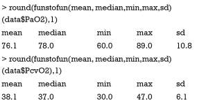
In big-data clinical study, there are numerous covariates under consideration. The first step is usually to take a look at these variables one by one. Suppose you want to have a look at the mean, median, range, and standard deviation of a variable. The traditional way is to execute functions one by one. Alternatively, you can combine these functions into a single one.

Sometimes, the summary() function contained in the base R package can fulfill the task of general description of variables. However, the output parameters are fixed. The funstofun() function overcomes this limitation that functions can be flexibly adapted to the needs of specific purpose.

Summary

The article provides a gentle introduction to data reconstruction and aggregating. It is common that the format of data output from case report form (CRF) does not meet the purpose of statistical analysis. In clinical research, variables are frequently measured repeatedly over the follow-up period. Such data can be displayed either in wide or long format. Transformation between these 2 forms can be challenging by hand. Fortunately, there are sophisticated packages in R environment. Data frame should firstly be melted and then casted to format that you want. Aggregation over unique combination of id variable is also allowable. Additionally, the article also introduces 2 functions colsplit() and funstofun() that may be useful in some situations.

Acknowledgements

None.

Footnote

Conflicts of Interest: The author has no conflicts of interest to declare.

References

1. Twisk JW. Applied longitudinal data analysis for epidemiology: a practical guide. Second edition. Cambridge, England: Cambridge University Press, 2013:321.
2. Wickham H. Reshaping data with the reshape package. Journal of Statistical Software 2007;21:1-20.