Variable selection with stepwise and best subset approaches

Introduction

The previous article introduces purposeful selection for regression model, which allows incorporation of clinical experience and/or subject matter knowledge into statistical science. There are several other methods for variable selection, namely, the stepwise and best subsets regression. In stepwise regression, the selection procedure is automatically performed by statistical packages. The criteria for variable selection include adjusted R-square, Akaike information criterion (AIC), Bayesian information criterion (BIC), Mallows’s Cp, PRESS, or false discovery rate (1,2). Main approaches of stepwise selection are the forward selection, backward elimination and a combination of the two (3). The procedure has advantages if there are numerous potential explanatory variables, but it is also criticized for being a paradigmatic example of data dredging that significant variables may be obtained from “noise” variables (4,5). Clinical experience and expertise are not allowed in model building process.

While stepwise regression select variables sequentially, the best subsets approach aims to find out the best fit model from all possible subset models (2). If there are p covariates, the number of all subsets is 2^p. There are also varieties of statistical methods to compare the fit of subset models. In this article, I will introduce how to perform stepwise and best subset selection by using R.

Working example

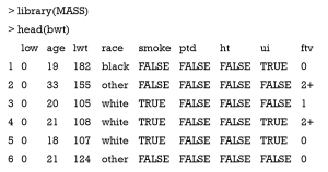
The working example used in the tutorial is from the package MASS. You can take a look at what each variable represents for.

The bwt data frame contains 9 columns and 189 rows. The variable low is an indicator variable with “0” indicates birth weight >2.5 kg and “1” indicates the presence of low birth weight. Age is mother’s age in years. The variable lwt is mothers’ weight in pounds. Race is mother’s race and smoke is smoking status during pregnancy. The number of previous premature labor is plt. Other information includes history of hypertension (bt), presence of uterine irritability (ui), and the number of physician visits during the first trimester (ftv).

Stepwise selection

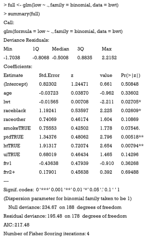
We can begin with the full model. Full model can be denoted by using symbol “.” on the right hand side of formula.

As you can see in the output, all variables except low are included in the logistic regression model. Variables lwt, race, ptd and ht are found to be statistically significant at conventional level. With the full model at hand, we can begin our stepwise selection procedure.

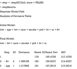
All arguments in the stepAIC() function are set to default. If you want to set direction of stepwise regression (e.g., backward, forward, both), the direction argument should be assigned. The default is both.

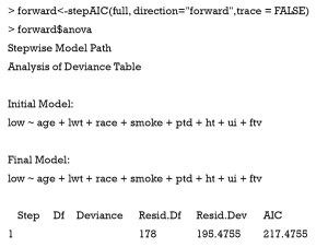
Because the forward stepwise regression begins with full model, there are no additional variables that can be added. The final model is the full model. Forward selection can begin with the null model (incept only model).

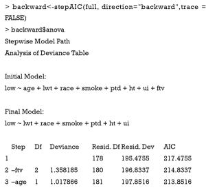
The backward elimination procedure eliminated variables ftv and age, which is exactly the same as the “both” procedure.

Different criteria can be assigned to the stepAIC() function for stepwise selection. The default is AIC, which is performed by assigning the argument k to 2 (the default option).

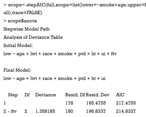
The stepAIC() function also allows specification of the range of variables to be included in the model by using the scope argument. The lower model is the model with smallest number of variables and the upper model is the largest possible model. Both upper and lower components of scope can be explicitly specified. If scope is a single formula, it specifies the upper component, and the lower model is empty. If scope is missing, the initial model is the upper model.

When I specify the smallest model to include age variable, it will not be excluded by stepwise regression (e.g., otherwise, the age will be excluded as shown above). This function can help investigators to keep variables that are considered to be relevant by subject-matter knowledge. Next, we can have more complicated model for stepwise selection.

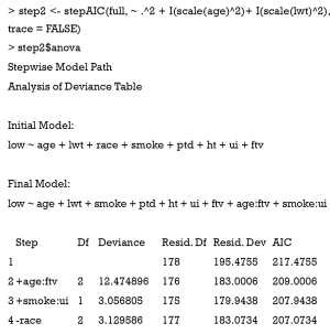
Recall that “^” symbol denotes interactions up to a specified degree. In our case, we specified two-degree interactions among all possible combinations of variables. Elements within I() are interpreted arithmetically. The function scale(age) centers variable age at its mean and scales it by standard deviation. “~ .^2 + I(scale(age)^2)+ I(scale(lwt)^2)” is the scope argument and a single formula implies the upper component. The results show that the interaction between age and ftv, smoke and ui are remained in the final model. Other interactions and quadratic terms are removed.

Best subset regression

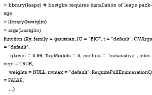
Best subset regression selects the best model from all possible subsets according to some goodness-of-fit criteria. This approach has been in use for linear regression for several decades with the branch and bound algorithm (6). Later on, lawless and Singhal proposed an extension that can be used for non-normal error model (7). The application of best subsets for logistic regression model was described by Hosmer and coworkers (8). An R package called “bestglm” contains functions for performing best subsets selection. The bestglm() employs simple exhaustive searching algorithm as described by Morgan (9).

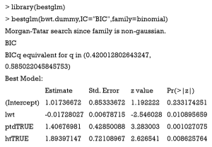
Xy is a data frame containing independent variables and response variable. For logistic regression model when family is set to be binomial, the last column is the response variable. The sequence of Xy is important because a formula to specify response and independent variables are not allowed with bestglm() function. We can move the response variable low to the last column and assign a new name to the new data frame. The IC argument specifies the information criteria to use. Its values can be “AIC”, “BIC”, “BICg”, “BICq”, “LOOCV” and “CV” (10).

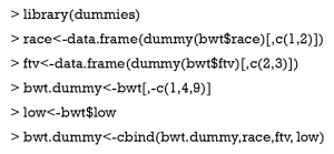
Furthermore, factors with more than two levels should be converted to dummy variables. Otherwise, it returns an error message.

To create dummy variables for factors with more than two levels, we use the dummies package. The dummy() function passes a single variable and returns a matrix with the number of rows equal to that of given variable, and the number of columns equal to the number of levels of that variable. Because only n-1 dummy variables are needed to define a factor with n levels, I remove the base level by simple manipulation of vectors. Finally, a new data frame containing dummy variables is created, with the response variable in the last column.

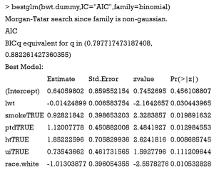
The model selection by AIC always keeps more variables in the model as follows.

Readers can try other options available in bestglm() function. Different options may result in different models.

Summary

The article introduces variable selection with stepwise and best subset approaches. Two R functions stepAIC() and bestglm() are well designed for these purposes. The stepAIC() function begins with a full or null model, and methods for stepwise regression can be specified in the direction argument with character values “forward”, “backward” and “both”. The bestglm() function begins with a data frame containing explanatory variables and response variables. The response variable should be in the last column. Factor variables with more than two levels should be converted before running bestglm(). The dummies package contains good function to convert factor variable to dummy variables. There are varieties of information criteria for selection of the best subset model.

Acknowledgements

None.

Footnote

Conflicts of Interest: The author has no conflicts of interest to declare.

References

1. Hocking RR. A biometrics invited paper. The analysis and selection of variables in linear regression. Biometrics 1976;32:1-49. [Crossref]
2. Hosmer DW Jr, Lemeshow S, Sturdivant RX. Applied Logistic Regression. Hoboken: John Wiley & Sons, Inc, 2013.
3. Harrell FE. Regression modeling strategies: with applications to linear models, logistic regression, and survival analysis. New York: Springer-Verlag New York, 2013.
4. Freedman DA. A note on screening regression equations. The American Statistician 1983;37:152-5.
5. Flack VF, Chang PC. Frequency of selecting noise variables in subset regression analysis: a simulation study. The American Statistician 1987;41:84-6.
6. Furnival GM, Wilson RW. Regressions by leaps and bounds. Technometrics 1974;16:499-511. [Crossref]
7. Lawless JF, Singhal K. ISMOD: an all-subsets regression program for generalized linear models. II. Program guide and examples. Comput Methods Programs Biomed 1987;24:125-34. [Crossref] [PubMed]
8. Hosmer DW, Jovanovic B, Lemeshow S. Best subsets logistic regression. Biometrics 1989;45:1265-70. [Crossref]
9. Morgan JA, Tatar JF. Calculation of the residual sum of squares for all possible regressions. Technometrics 1972;14:317-25. [Crossref]
10. McLeod AI, Changjiang X. bestglm: best subset GLM.–R package ver. 0.34. 2014. Available online: https://cran.r-project.org/web/packages/bestglm/bestglm.pdf